|
KTH Royal Institute of Technology |
|
VHF/UHF Uplink Solutions for Remote Wireless Sensor Networks |
|
The purpose of this thesis was to compare alternative wireless links for transfer of data from sink motes of remote wireless sensor networks to a central repository. We discussed a few different protocol stacks to be implemented in the WSN uplink gateway and a few implementation environments based on open source software and low-power hardware. To facilitate measurements and experimental validation, some of the alternatives have been implemented. Experiments have been made using radio amateur frequencies, the 144 MHz band (VHF) and the 434 MHz band (UHF). The parameters studied include throughput, range, power-requirements, portability and compatibility with standards. |

|
Alp Sayin 21 May 2013
|
The purpose of this thesis was to compare alternative wireless links for transfer of data from sink motes of remote wireless sensor networks to a central repository. A few different protocol stacks to be implemented in the WSN (Wireless Sensor Network) uplink gateway and along with them a few implementation environments based on open source software and low-power hardware were discussed. To facilitate measurements and experimental validation, some of the alternatives have been implemented. Experiments have been made using two of the amateur radio bands, the 144 MHz band (VHF) and the 433 MHz band (UHF). The parameters studied include throughput, range, power-requirements, portability and compatibility with standards.
Using different protocol stacks, different bands and sometimes different hardware 5 solutions were designed, implemented, tested and experimented with. Namely these solutions are called Radiotftp, Radiotftp_process, Radiotunnel, Soundmodem and APRX in this thesis.
After the implementation phase, there was an open-field experimentation to measure the aforementioned parameters. The tests were conducted in Riddarholmen, Stockholm of Sweden. These open-field experiments helped us obtain real-life measurements about power, throughput, stability etc. Experiments were conducted in a range of from a minimum of 2 meters to a maximum of 2.1 kilometers with some of the solutions.
In the end, some of these solutions proved themselves to be viable for the purpose of data communications for remote wireless sensor networks. Radiotftp gave the best throughput in both bands where it proved itself to be difficult to develop further applications. Radiotftp_process removed the necessity for a Linux running gateway machine but it was unable to work with faster baud rates. Radiotunnel opened up the path for a range of network applications to use radio links, but it also proved that it was unstable. On the other hand Soundmodem and APRX which were based on standard and open-source software proved that they were stable but rather slow. It was proven that every approach to problem has its advantages and disadvantages from different aspects such as throughput, range, power-requirements, portability and compatibility.
Acknowledgements
First of all, I would like to thank my project supervisors Bjorn Pehrson and Robert Olsson. They were the first people to introduce me to this interesting branch of wireless communications. Before this project I -literally- had no idea such a world even existed. Being a radio amateur himself Bjorn was always there to introduce me to new topics and technologies about the project. I was getting new information almost every week and I am very thankful about it. On the other hand Robert always helped me about the technical details, he taught me to ‘hack’ into the stuff that I didn’t know about. Later on, I found out that this is the only tool that I’ll need in real life, whether it be research topics or company projects.
Secondly, I would like to thank my examiner Hakan Olsson for his extended patience and understanding during my last semesters. Although we couldn’t be in contact that much, I always felt his support and belief for my success.
Finally, since this is the documentation of the end of my Master’s studies, I would like to thank to all people who have somehow supported me during the years I’ve spent in Sweden. These people are my family and my friends.
Shortly I would like to mention their names; my parents, Meral Sayin and Erol Sayin who have supported me both financially and morally during my studies. They were the ones I held onto when I thought of quitting for a couple of times. My friends from Turkey; Melih Cinalioglu, Berkay Karatan, Berkay Balci and Burak Kilic, somehow they were always online whenever I needed an old friend to talk to. They were my online companions during the long nights of studies. My friends in Sweden; Moysis Tsamsakizoglou, Stefano Vignati, Theodor Stana, Bahar Palabiyik, Mert Karadogan and many more… In my belief without these people my Sweden experience would be a total disaster. I owe it to them for all the great times we had.
If I start writing all the names in my head, this part of the thesis would probably be longer than the thesis itself, so I stop here. But people who have helped me even a little should consider themselves thanked here with great gratitude.
All in all, I am very thankful to all the people who have somehow helped me or been there for me during these years. Even though this thesis has my name on it, I owe it to them, so I humbly present it to them.
Alp Sayin
May 2013
10.1.1 Experiments with radiotftp
10.1.2 Experiments with radio_tunnel & soundmodem
10.1.3 General Experiments with Bim2A and UHX1
10.1.4 General Experiments for UHX1 (Optional)
16.1 State Machines and Code Segments
18.1.1 Data Collected in 144 MHz Experiments (UHX1)
18.1.1.1 Single Packet Transaction Experiments (127 Bytes)
18.1.1.2 Many Packet Transaction Experiments (2 Kbytes)
18.1.2 Data Collected in 434 MHz Experiments
18.1.2.1 Single Packet Transaction Experiments (127 Bytes)
18.1.2.2 Many Packet Transaction Experiments (2Kbytes)
19.1 Schematics and PCB Designs
Figure 1 Resulting branches in the project after design decisions
Figure 2 Resulting solutions after hardware decisions
Figure 3. System diagram for radiotftp solution
Figure 4 System diagram for radiotftp_process solution
Figure 5 Size footprint of Fibonacci application with radiotftp_process
Figure 6 System diagram for radio_tunnel solution
Figure 7 System diagram for soundmodem solution
Figure 8 Soundmodemconfig utility configuration options
Figure 9 Yaesu FT8900R Data port signals
Figure 10 Audio leveler and PTT controller card
Figure 11 Soundmodemconfig utility channel settings
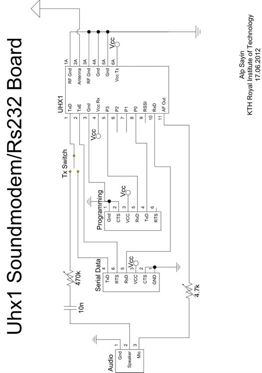
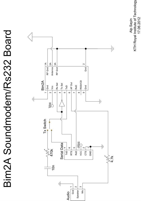
Figure 12 Simple audio leveler and push-to-talk circuit
Figure 13 System diagram for APRS solution
Figure 14 Simple configuration file for aprx,
Figure 15 aprs_telemetrit usage
Figure 16 Map of Gamla Stan Experiments
Figure 17 Transfer time plots for single packet delivery
Figure 18 Transfer time plots for many-packet delivery
Figure 19 Error rate plots for single packet delivery
Figure 20 Error rate plots for many-packet delivery
Figure 21 Bitrate plots for single packet delivery
Figure 22 Bitrate plots for many-packet delivery
Figure 23 Pseudocode showing the workflow of the IP stack implementation of radiotftp
Figure 24 Radiotftp_process Receive FSM diagram
Figure 25 Radiotftp_process send FSM diagram
Figure 26 Sample Contiki Process computing Fibonacci Series
Figure 27 Code segment from tun_alloc.c, demonstrating the opening procedure of a Tun device
Figure 28 Ping responder code segment from tunclient.c
Figure 29 A simple fix to disable automated telemetry messages of aprx.
Figure 30 A simple shell script to automate the transmission of data as APRS telemetry
Table 1 Distances of test points to base station in Riddarholmen
Table 2 Average transfer times with minimum distance between transceivers
Table 3 RSSI readings from various locations with UHX1 and Bim2A
Table 5 Sample event log extract
Table 6 Results of transfer experiments with 127 bytes in location 0.
Table 7 Results of transfer experiments with 127 bytes from location 1.
Table 8 Results of transfer experiments with 127 bytes from location 2.
Table 9 Results of transfer experiments with 127 bytes from location 3.
Table 10 Results of transfer experiments with 127 bytes from location 4.
Table 11 Results of transfer experiments with 127 bytes from location 5.
Table 12 Results of transfer experiments with 127 bytes from location 6.
Table 13 Results of transfer experiments with 127 bytes from location 7.
Table 14 Results of transfer experiments with 2 kbytes in location 0.
Table 15 Results of transfer experiments with 2 kbytes from location 1.
Table 16 Results of transfer experiments with 2 kbytes from location 2.
Table 17 Results of transfer experiments with 2 kbytes from location 3.
Table 18 Results of transfer experiments with 2 kbytes from location 4.
Table 19 Results of transfer experiments with 2 kbytes from location 5.
Table 20 Results of transfer experiments with 2 kbytes from location 6.
Table 21 Results of transfer experiments with 2 kbytes from location 7.
Table 22 Results of transfer experiments with 127 bytes in location 0.
Table 23 Results of transfer experiments with 127 bytes from location 1.
Table 24 Results of transfer experiments with 127 bytes from location 2.
Table 25 Results of transfer experiments with 127 bytes from location 4.
Table 26 Results of transfer experiments with 2 kbytes in location 0.
Table 27 Results of transfer experiments with 2 kbytes from location 1.
Table 28 Results of transfer experiments with 2 kbytes from location 2.
Table 29 Results of transfer experiments with 2 kbytes from location 4.
ADC – Analog to Digital Converter
AFSK – Audio Frequency Shift Keying
APRS – Automatic Packet Reporting System
CD – Carrier Detect
CSMA – Carrier Sense Multiple Access
FCS – Frame Check Sequence
FSK – Frequency Shifted Keying
FSM – Finite State Machine
IEEE – Institute of Electrical and Electronics Engineers
GNU - GNU’s not Unix
GPLv2 – General Public License version 2
GPRS – General Packet Radio Service
IP – Internet Protocol
KTH – Kungliga Tekniska Högskolan
MCU – Microcontroller Unit
MTU – Maximum Transmission Unit
NBFM – Narrow Band Frequency Modulation
NMT – Nordic Mobile Telephone
OS – Operating System
OSI – Open Systems Interconnection
RF – Radio Frequency
RSSI – Receive Signal Strength Indicator
SLIP – Serial Line IP
TCP – Transmission Control Protocol
TFTP – Trivial File Transfer Protocol
TNC – Terminal Node Controller
TSLab – Telecommunication System Laboratory
UART – Universal Asynchronous Receiver/Transmitter
UDP – User Datagram Protocol
UHF – Ultra High Frequency
UI – Unnumbered Information
VHF – Very High Frequency
The main author of this thesis is Alp Sayin, who is a second year System-on-Chip Design student. All thesis work was completed by him. This includes codes, documentations, reports and hardware designs. The thesis was built on previous works on this field from sources like published papers and amateur radio community.
The supervisors are Robert Olsson and Björn Pehrson from KTH. The examiner is Hakan Olsson from KTH.
The context of this thesis is the work at TSLab on Open Wireless Sensor Networks for environment monitoring. The system under development include sensors for environment monitoring connected to a sensor network node (mote), which can be interconnected to other similar motes to form a sensor network. This network can be placed in a remote area, with at least one of the motes being a sink node, i.e. connected to a gateway collecting the data and capable of delivering it via some sort of upstream connection to a central data repository. The purpose of this thesis is to explore different wireless upstream link options.
The WSN mote used in this thesis project is a Herjulf mote [1] based on the Atmel ATMega128RF-chip, which integrates an IEEE 802.15.4 [2] compliant 2.4 GHz radio transceiver, an MCU and an AD converter facilitating the connection of analog sensors. Motes broadcast packets with sensor data.
The mote software is based on the Contiki operating system [3].
The following sections discuss different aspects of the uplink from the WSN gateway and the experiments conducted to facilitate comparisons.
Detailed information about the structure of this report can be found in the following Thesis Structure chapter in page 13.
A sensor network is a networked system of interconnected measurement nodes communicating and reporting their measurement data to a central repository. In a wireless sensor network (WSN) these nodes are connected to each other wirelessly, and the nodes are usually low-power microcontroller units with no significant memory storage.
In more detail, a WSN is built of nodes (or motes) of from a few to several hundreds or even thousands, where each node is connected to one (or several) sensors. Each such sensor network node has typically several parts: a radio transceiver with an internal antenna or connection to an external antenna, a microcontroller, an electronic circuit for interfacing with the sensors and an energy source, usually a battery or an embedded form of energy harvesting (e.g. solar panels). Size and cost constraints on sensor nodes result in corresponding constraints on resources such as energy, memory, computational speed and communications bandwidth. The topology of the WSNs can vary from a simple star network to an advanced multi-hop wireless mesh network. The propagation technique between the hops of the network can be routing or flooding [4].
In our case the motes included sensors for synoptic weather data, soil moisture and drinking water quality parameters, such as turbidity, acidity and redox-potential. Some motes also contain solar panels to measure the solar power efficiency through the day and sensors monitoring the voltage and temperature of connected batteries used as energy source.
The MCU currently used for mote experiments is an Atmel ATMega128RFA1 [5]. It integrates an MCU, ADC and RF-module in one chip. In deep sleep it consumes about 1 uA. Small solar panels are used as power source. Instead of chemical batteries, ultra-capacitor batteries in different sizes are used as power storage. The motivation for this choice is that they have much longer lifetime and are not affected by operating temperature. Two different operating systems dedicated for wireless sensor networks have been explored [6], Contiki [7] and TinyOS [8]. Contiki-Os was found more beneficial for the work in TSLab. The Contiki capabilities for multi-tasking and its internal communication stacks were found much more powerful than that of TinyOS. Furthermore the necessity to learn the new programming language used in TinyOS, NesC, made it less preferable, due to the time requirements [9] [10].
The communication between the sensor network nodes is supplied by internal radios working on 2.4 Ghz band using the IEEE 802.15.4 protocol [2]. This is a low power communication option which usually allows 10-20 meters of range with an average 250 kbit/s raw data rate. In our case, the nodes wake up according to a schedule, broadcast messages with sensor data that can be captured by the sink node and goes back to deep sleep. On top of the IEEE 802.15.4 link protocol the Contiki’s Rime protocol is used to broadcast [11].
A Herjulf mote automatically becomes a sink mote when connected via a TTL/USB converter to a USB port of a gateway.
The gateway used in this thesis project is the Alix [12] board running the Bifrost-Linux [13] operating system which is optimized for routing. The Voyage-Linux [14] operating system is also sometimes used due to its easiness for adding packages. Search for something more power-lean than the Alix board is going-on, for example a Raspberry Pi [15] with Debian inside [16].
The gateway software used to fetch measurement data from the sinknode over the USB interface into the gateway is called sensd [17]. It stores the data from received packets in a file from which it is to be sent upstream to the central repository.
Uplinks can be implemented in different ways, including
· Cabled connection (copper or optical fibre), if available
· Terrestrial wireless connection, either using a data service offered by a cellular mobile network operator or using a dedicated terrestrial wireless link on a suitable frequency
· Satellite connection
· Some sort of physical transport of data (e.g. based on Delay Tolerant Networking using wireless phones as data carriers [18] ).
The purpose of this thesis is to explore the dedicated terrestrial wireless link options.
The main problem of this project is to get the collected data out from the sink mote of a wireless sensor network to a remote repository with internet access. The objective of this thesis project is exploring the tradeoffs coming with the use of
a. 434 MHz and 144 MHz frequencies and associated protocol stacks to optimize the range and QoS (throughput, data rate, error rate).
b. Different hardware and software solutions, from dedicated hardware solutions to software defined radio links to optimize power consumption and flexibility.
The overarching goal is to add IP over a VHF/UHF software defined radio link interface to Alix/Bifrost gateway. And while achieving this goal, mobility of the design will also be taken into consideration, meaning that presumed outcome of the thesis project is a portable device that uses serial port and not so dependent on the connected platform.
Similar environmental wireless sensor network projects have been known to use off-the-shelf solutions[19][20]. A 900 MHz radio modem called FreeWave Ranger is used in these projects. This device can give 115.2 kbps throughput with about 90 km range with clear line of sight [21].
Some other similar projects use 2.4 GHz 802.11 links with directed antennas [22]. By using directed antennas, these projects acquired a longer range. But they were only able to reach about 300 meters. And even the researchers in that project decided to leave their Wi-Fi gateway solution due to two main reasons; excessive power consumption and the overhead caused by TCP/IP and 802.11b link.
Also some wireless sensor network projects have tried the option of GPRS modems, but decided that it was not providing a stable connection [23]. In more detail, they have found out that GPRS modems tend to lock up after extended periods of time (2-4 days) and can be recovered only by re-cycling power to them. According to the researchers GPRS modems are generally not robust enough to run long-term outdoor applications.
One of the projects decided to leave the data in the sink and retrieve it manually [24]. In this implementation of the WSN, each node has its SD card storage where they store their data. And this data can be queried from the sink node when it’s necessary. This implementation was chosen to reduce the complexity of the system, and it was found not necessary to relay the data since the researchers were also present on the field during the time of measurements.
Unfortunately the academic study brought up no specialized projects focusing on the uplink itself. All the projects mentioned above were about the implementation of the wireless sensor network rather than the uplink. But they were still explaining their uplink implementations, which proved to be useful.
Primary goal of this thesis project was to produce a feasible, minimum hardware, low-cost, low-power, long range solution to the problem of getting the sensor data out from the sink mote to a remote repository. Secondary goal was to implement IP over the same solution, so that existing user programs, or newly developed programs could be used over this link. When this thesis project was finished, it was planned to have at least one hardware/software solution which will be plugged into the sensor network and the remote repository which would carry the sensor data reliably.
Section 1 tells about the background of the project, giving details about the situation at hand before the project started. Section 2 explains the problem statement. Section 3 gives brief information about the academic studies regarding the problem. And Section 4 tells about the goals of this thesis relating to the problem. Further on, Section 6 tells about the method that was used in this project. Section 7 gives details about the literature study before telling about the design decisions which is in Section 8. After the design decisions; in Section 9 implementation details are presented. After, in sections 10 and 11, the experiment plan and the data gathered in experiments are presented. Finally in sections 12 and 13, the conclusions and possible further work is given. And finally, references can be found in section 14.
Before starting the project, a literature study has been conducted to understand the problem, to know about the communication protocols and stacks and to understand how packet radio works. After this study, the metrics of the problem has been defined to have a clearer grasp of the problem and goals. Later on, existing solutions to the problem has been explored to see if they fulfill the requirements. This research included both general literature and academic resources. After seeing that existing solutions were not enough, new solutions to the problem were generated approaching the problem from its uncovered requirements. The parts until this point structured the theoretical study phase of the thesis study.
Then, a measurement model is created to have a basis to compare solutions at hand. This model defines what to measure and how to measure the key parameters.
After the measurement model phase, there came the implementation phase which was done in three steps: architecture design, application design and the implementation itself. In architecture design phase the supporting hardware and software was designed. In the application design and implementation phases, the application was designed and implemented.
After the implementation phase, experiment plan was executed and data were collected. Then, after the interpretation of the collected data, conclusions were deduced by discussing the results.
There are many possible communication protocols and protocol stacks that can be used for uplink communication. While the project requirements only determined the use of a single type of physical layer, the protocol selection for rest of the layers -data link, network, transport and application- was up to the author. Below are the discussions for different layers and different protocols.
The physical layer in this project is based on wireless streaming, and VHF/UHF bands are used. For VHF, the used amateur band is 144 MHz (i.e. 2 meter band), and for UHF based amateur radio the band is 433 MHz (i.e. 70 centimeter band). For these bands, there are rules of the amateur radio communications. These rules are generally the same, but may differ from country to country. An example of these rules for United States can be found in [25]. One important general rule is that the transmitter must periodically send out the call-sign of the operator during transmissions.
On these frequency bands, we have the ability to transmit audio with a maximum of 9600 Hz sample rate depending on the underlying hardware. Between the modulation options, there are two popular choices, one of them is the bi-phase encoding (Manchester) [26] and the other is AFSK (i.e. 1200 baud Bell Modem) [27].
The “soundmodem” [28] software at hand was able to generate AFSK signals for us, but on the other hand the Radiometrix devices were not proven to work with that yet. So at the beginning of the project the Radiometrix devices were only compatible with the digital feed.
It should also be noted that, although Radiometrix devices work the same way, there are different constraints regarding the maximum possible baud rate that could be used. In 70 cm band (Radiometrix Bim2A [29]), the maximum possible baud rate is 19.2 kbits/sec without overwhelming the packet error rate, whereas in 2 m band (Radiometrix UHX1 [30]) the maximum possible baud rate is 2.4 kbits/sec [31].
For the data link protocol, the most important part was the frame format. For data link layer three possible protocols were considered. These are Ethernet, IEEE 802.15.4 and AX.25 [32] [2] [33].
An Ethernet frame consists of at least 18 bytes disregarding the preambles and delimiters. It provides 6 byte source and destination addresses, 2 byte length field, 4 byte 32-bit CRC checksum field and a maximum of 1500 byte payload.
An 802.15.4 Data frame consists of at least 21 bytes if full addressing mode is used. It has 2 bytes of frame control field, 1 byte of sequence number, 4-20 bytes of address information and 2 bytes of frame check sequence.
An AX.25 Unnumbered Information frame consists of 18 bytes. It provides 7 byte source and destination addresses. In addition it has 1 byte control field, 1 byte protocol identifier field and 2 bytes of CRC checksum field. AX.25 is a link-layer protocol which is defined to reliably deliver data over two amateur radio stations [33]. Although AX.25 is said to be a link-layer protocol, it also has utilities for routing and connection-oriented transfers [33]. The simplest form of AX.25 frames are the UI frames. These frames are similar to the UDP/IP frames. AX.25 defines a framing format for packets, protocols etc. But it does not define a physical layer, meaning that it can be built upon any type of physical connection, which will be demonstrated later in this thesis.
For network layer, IP or APRS was considered as possible options. So in the end there were 3 possible options: IPv4 [34], IPv6 [35] or APRS [36]. It should be noted that APRS is not actually an OSI compatible network layer; it actually covers network, transport and application layers. But since it can be used on top of a data link layer, it was also discussed under this title.
An IPv4 header consists of at least 20 bytes. The most important information for us in this header are the 4 byte source and destination IP addresses, the 2 byte header checksum, 2 byte total length field, and 1 byte time to live field.
An IPv6 header consists of at least 40 bytes. The most important information for us in this header are the 16 byte source and destination IP addresses, the 2 byte payload length field and the single byte hop limit field which is the equivalent of time-to-live field in IPv4 header.
APRS, Automatic Packet Reporting System is a system developed to deliver APRS messages to a centralized database [37]. It can also be used to deliver messages between stations. An APRS packet usually lies on top of an AX.25 layer. It makes use of the AX.25 UI (unnumbered information) frames. It doesn’t have a specific header, except for the AX.25 source and destination call signs which are already included in AX.25 header. They are actually simple text messages with a maximum length of 256 bytes including the AX.25 headers [36].
Like it is for many other systems, the choice of transport layer was between UDP [38] and TCP [39]. The main differences between UDP and TCP will not be discussed here. But the main difference from the author’s perspective was that UDP was easier to implement compared to TCP. But since TCP provides reliable connection, it would need more effort to design and implement the application layer. But in most cases the transport layer to be used is determined by the application to be used (e.g. FTP [40], HTTP [41], TFTP [42]).
UDP (User Datagram Protocol) is most basic transport layer which is on top of IP; it only provides application multiplexing via the use of port numbers [38]. Programmers who plan to use UDP as transport layer should cover the cases for packet loss and erroneous packets. It is often easy to implement but difficult to use.
TCP (Transmission Control Protocol) gives the user the ability open reliable data streams called sockets [39]. While using TCP, a programmer doesn’t have to consider the possibility of packet losses or errors in packets since TCP takes care of that. Unlike UDP, it is more difficult to implement TCP but due to its features, it is an easier transport layer to build applications upon.
Regarding IP based network protocols; in Linux based systems TUN/TAP [43] devices can be used to read in/write out raw IP data from/to user programs. These virtual network kernel devices allow users to write their own network drivers without going deep into the Linux kernel. This allows a developer to tunnel the IP packets from user programs to do whatever they like for example redirect them to a radio device.
APRS also has some routing utilities which resembles functionality of a transport layer. APRS messages are carried and routed with repeaters called digi-peaters [44]. When an APRS message is relayed, the digi-peater adds its call-sign to the message so that it doesn’t pass through that station again. But apart from this, APRS transportation is based on flooding [45]. APRS also has some special call-signs to designate a direction to the messages, so that location-aware stations can ignore and drop the message.
Except TCP and UDP there is one interesting protocol that is available, which is called CoAP. CoAP, the Constrained Application Protocol is a transfer protocol designed for half-duplex and/or low bandwidth channels [46]. It is a transport layer protocol, not an application layer protocol. It works on two types of messages; requests and responses. And it is a RESTful [47] protocol which makes it more compatible with HTTP. It also normally depends on UDP or other unreliable transport layer, and it has its own mechanisms to avoid congestion and packet loss. Its congestion avoidance mechanism is exponential back-off. One important thing is CoAP does not assume anything about what-duplex the underlying channel is. On the other hand, a programmer can tune his application to use CoAP on a half-duplex channel very efficiently. One of its advantageous properties is to be able to mark messages as `confirmable` or `non-confirmable`. Which -for example in a sensing application- could be used in such a way: If a reading does not change with respect to the previous reading, the new reading could be sent as non-confirmable, spending less bandwidth and resources and so on. Contiki-OS also has a low-power implementation of CoAP which might be used [48].
There are many possible application layers that could be used to transfer files but we explain the most popular ones here, which are HTTP, TFTP and APRS. HTTP works over TCP/IP, TFTP is usually works over UDP/IP but can also work with TCP/IP and APRS works over connection-less AX.25 [41][42][36].
HTTP is the protocol that is widely used in today’s world-wide-web to exchange files between clients and servers. It provides a simple request/response protocol, but can be used for higher functionality access and/or modify any kind of resource.
TFTP is a very old file transfer protocol from the times of early TCP development. It was designed to simply transfer files without complexity. TFTP has some specific limitations to itself; e.g. file size cannot be larger than 4 gigabytes, or there is no handshake to finish a transfer.
APRS is generally used for weather and location reporting, and also used for messaging between amateur radio stations. It also has a telemetry reporting functionality for users who want to report any kind of measurement data. This functionality is usually popular with the amateur ballooners who collect different kinds of data from air or from their balloon. The data server and user interface for APRS system –namely aprs.fi website- has a feature to plot these measurements data for users instead of just showing it in a table.
For hardware there are all sorts of interesting radio options. Usually packet radio is implemented via a TNC (Terminal Node Controller) and a regular handheld or movable radio station from brands like MAAS or Yaesu [45]. In this sort of setup AX.25 packet generation, modulation and PTT control is handled by the TNC and transmission and reception is handled by the radio.
One interesting possible choice of hardware is the use of dedicated radio modules like Radiometrix devices. These devices are at most credit card sized modules which has the same properties as a radio except for the natural user interface such as speakers, microphone and/or buttons. These devices –depending on the model- are completely programmable via their digital ports and support the transmission and reception of digital signals as well as analogue signals. Like regular radios most of the models do not provide full-duplex channels but half-duplex channels. The most interesting models from the Radiometrix family are the Bim2A [29] and UHX1 [30].
The Bim2A model is a fixed frequency UHF transceiver with fixed transmission power of 10 mW. This model can be easily used by connecting it to a serial port of a computer or a microprocessor. Or it can also be used to send and receive analogue signals, but this requires a sound card or an ADC/DAC couple and some software or hardware processing to convert the signals into data. In any case the PTT is signaled via assertion of the TX enable pin. It is again up to the user how to assert this signal, but the easiest suggested method is using the RTS flow control signal of a serial port.
The UHX1 model is a multi-frequency VHF transceiver with programmable transmission power (1 mW to 500 mW) and with programmable frequency (144 MHz to 146 MHz). Except for the extended programmability the use of UHX1 is very similar to Bim2A. The easiest way to use it is to connect it via a serial port. But the ability to change frequency and power gives the user more flexibility about implementing a link (i.e. frequency hopping, power decreasing when necessary etc.).
As previously mentioned the goals included the outcome of the project to have low power consumption, minimum hardware requisite (low financial cost) and long range. Here, we defined these metrics and measurement models for these metrics.
The maximum transmission power of IEEE 802.15.4 packets in the wireless sensor network is 2.5 milliWatts [5]. And from the related works we also learned that usual 802.11 Wi-Fi links use 100 milliWatts of transmission power [49]. So the author decided to set 2.5 mW as lowest possible transmission power and 100 mW as the highest possible transmission power for the uplink.
The hardware requirements were metricized in means of financial cost. So every chip, cable and PCB production cost was a negative point for the minimum hardware goal.
The range is normally very dependent on the transmission power, but in this project we decided that range metric should be done regarding the same transmission power for different solutions. Apart from that, the personal experiments of Robert Olsson showed a 200 meter range with IEEE 802.15.4 protocol with 2.5 mW transmission power with directed antennas. Therefore author decided that for 10 mW 400 meters were the minimum acceptable range by using the simple power vs. range relation (range is directly proportional to the square root of transmission power). There was no maximum range specified for this project since the goal was to reach as far as possible.
8 Design Decisions
On the WSN side, the decision was to use a topology with a sink node connected to, or integrated with, the uplink gateway. All WSN nodes use the Rime Protocol over IEEE 802.15.4 protocol stack and are implemented using the ATMega128RFA1 MCU with integrated radio and Contiki as OS.
On the uplink side, the decision was to try two different Radiometrix radio components, Bim2A (434 MHz) and UHX1 (144 MHz) [29] [30]. These radios are both NBFM radios. They support feeding a digital data stream directly or feeding a high level linear signal such as an AFSK modulated signal, into their inputs. Using a digital stream means that the radio component can be connected via a serial port, while using a modulated signal means interfacing via a separate hardware modem (e.g. TNC) or via a soundcard and a soft-modem (e.g. soundmodem). Also in the development process instead of single-chip radio solutions, handheld [50] or portable radio stations [51] were also used.
In all cases TX/RX switching was done via a serial port’s RTS signal. Using a digital feed is less complex, which facilitated the interconnection of the uplink gateway and WSN the sink node. Using an analog feed requires a separate modem or more software and processing power, but can be adapted to existing standards more easily.
The choice of OS/computer/processor when implementing the uplink gateway was a tradeoff between ease of demonstration and performance optimization.
When using the digital input in the uplink radio, it was also interesting to explore if the upstream gateway may be possible to implement under Contiki-Os, which is demonstrated later in this section in hardware decisions.
When using a dedicated gateway, the stepwise refinement chosen was as below to speed up the development process;
1. Ubuntu/Laptop
2. Voyage/Alix
3. Bifrost/Alix.
Below are the design decisions made regarding the communication protocols and their discussions. And after that hardware selection has been made.
Since the project supervisors were interested in testing both frequency band which were mentioned before, the author decided to build the project to be compatible with both bands regarding the constraints that come with them. For this purpose the author decided to make the software parameterized to set the timings.
The project supervisors were also interested in testing both type of modulations (digital and analog). This decision was going to affect the future progress of the project since analog feeding required extra hardware and software relative to the digital feeding. Therefore the author decided not to select one type of modulation and decided to use whatever type of physical layer is feasible when the remaining design decisions are made. In any case later decisions were not affected by this decision due to the natural structure of the OSI Model [52].
For the link layer firstly the Ethernet frame format was considered. It provides the basic functionality of addressing and checksum to reliably transfer messages. Then 802.15.4 frames were also considered since it also provided the same functionality. The frames coming to the gateway are also 802.15.4 frames, and we thought we could use this fact to our advantage; the frames could directly be uploaded to the upstream.
But later it was decided that these options are not viable due to an amateur radio operating rule; whatever communication occurs within the amateur bands, the communique (the message) must include the call sign of the operator. AX.25 frames are actually exactly designed regarding this and many other rules. And it also provides the reliability with a 16-bit checksum. So for the link layer the AX.25 frame formatting was decided to be used from this point forward. And the fact that IP over AX.25 libraries existed and also APRS was also worked over AX.25 contributed to this decision.
For the network layer three options were possible, IPv4 IPv6 and APRS.
APRS messages are basically AX.25 UI packets with a special formatting. APRS was thought of transmitting messages between the gateway and the remote repository using station to station messaging system. Also instead of transmitting the collected data to a specific repository, transmitting the data to the APRS system via use of amateur radio software like “aprx” [53] and “xastir” [54] were explored. And in the end, “aprx” software was found to be more useful for our purposes due to its beaconing features that could be used to generate and transmit telemetry reports.
Regarding IPv4 and IPv6, at first it was considered that IPv6 would be more beneficial since mote addresses could be directly mapped to IPv6 addresses and due to its less number of redundant fields. But then due to its large header requirement –even with the discarded redundant fields- IPv6 was eliminated to have better data over header efficiency. For example the standard maximum packet size for AX.25 frames is 256 bytes. Therefore cutting 20 bytes from the header would give us an increase in the header efficiency of 8% in the network layer.
Regarding all possible network layers, the author and project supervisors decided to try and compare the possible outcomes with the choice of APRS vs. IPv4. So at this point of the project, there was a branching regarding the network layer. From this point forward next layers were considered differently for APRS and IPv4 case.
The decision between TCP and UDP was not a trivial choice. As mentioned before TCP was more difficult to implement but easier to use on the upper layers, and UDP was easier to implement and more difficult to use on the upper layers. Apart from this, most important factor in this decision was the overhead coming with the TCP. Also from the previous studies it was known that TCP would have a great overhead due to its features.
As mentioned before, virtual network kernel devices called TUN/TAP devices would allow the author to skip actually implementing TCP and would allow the usage of it directly. The “soundmodem” software would also allow the author to use TCP directly without actually having to implement it.
And for UDP, since it is a simple protocol, there wasn’t really a concern about how to implement, but a concern about the application.
At this point the author decided to try them both to observe the behavior of TCP in slow and half-duplex radio links. And also APRS –as mentioned before- was to be tried out too. So from this point forward there were three branches in the project that was going to test TCP/IPv4 over AX.25, UDP/IPv4 over AX.25 and APRS over AX.25.
Up to this layer, the project has already branched out to 3 different protocol stacks. For each of them a different application layer had to be chosen.
For the solution that was planned to use APRS over AX.25, there is no application layer to be chosen except for a client application to be run on since APRS also covers the application layer. And for client program two options were considered, “xastir” and “aprx”. As mentioned before “aprx” was chosen to be a better option for this project since, “aprx” was easily programmable to send out periodic telemetry messages. And it was also later discovered that “xastir” required a GUI to run.
For the TCP/IPv4 over AX.25 branch, HTTP was chosen as the application layer due its ease of use and due to accessibility to many libraries and software that supports it. And to serve the HTTP functionality, Apache [55] software was chosen as the server due its popularity and its ease of configuration. As the client application Wget [56] is chosen due to its many useful properties.
For the UDP/IPv4 over AX.25 branch, it was considered to write custom application layer software. But after the studies, the TFTP protocol [42] was discovered. The Trivial File Transfer Protocol was found to be perfect for the project’s requirements, and other options were left out such as FTP [40] or SFTP [57].
At this point of the project there are still three branches from the protocol stacks point;
· HTTP/TCP/IPv4/AX.25
· TFTP/UDP/IPv4/AX.25
· APRS/AX.25
More information about how these protocol stacks were implemented and/or used can be found in the Implementation Details in Section 15.
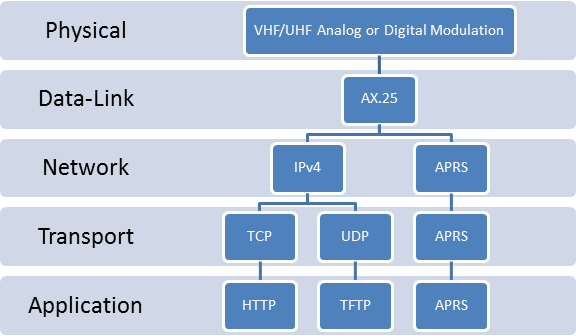
Figure 1 Resulting branches in the project after design decisions
For digital links it was seen that a regular (handheld or movable) radio is not fit for the job, so digital feeding was only possible with the use of Radiometrix devices. And for analogue feeding Radiometrix devices were not proven to be working during the project timeline, so a regular radio was decided to be used for the job (e.g. YAESU [51] or MAAS [50]).
For implementing a link with APRS over AX.25 the only possible way was found to be using the “soundmodem” software with “aprx” running with it. And for this purpose the conventional hardware selection is using a regular radio connected to a PC with a sound card and PTT is controlled via a serial port. So, for testing and implementation purposes a MAAS handheld radio connected to an Ubuntu computer via a USB audio card and a TTL/USB Uart cable [58] was decided to be used.
For implementing a link with TFTP over UDP/IP over AX.25 three possible options were considered; one of them was using the “soundmodem” software with linux network libraries using analogue modulation. Second one was using the TUN/TAP devices to create a kernel network interface and using serial port and therefore using digital modulation. And the last one was writing custom software with C using the serial port, therefore using digital modulation. Due to the implementation of APRS link, the “soundmodem” software was already going to be set up and tested, so author decided to leave out the option of “soundmodem”. The benefit of using TUN/TAP devices is that user programs can use TCP without dealing with any libraries or compatibility issues, and since we were aiming only to implement a UDP link, the author also decided to leave out this option. So we decided to go with the custom software option, so that the newly written software could be developed to be compatible for many more platforms and also requiring much less hardware (i.e. a Radiometrix device and a serial port connection). Also with full customization of the software the timings and any problems that could occur could be fixed by directly going into the code. At this point the author also decided to port this custom software to Contiki-OS for Atmega128RFA1 chip, so that its portability could be tested and verified.
For implementing a link with HTTP over TCP/IP over AX.25, two options were considered; one of them was using the network interface created by using the “soundmodem” software and to use some off-the-shelf HTTP server and client to test the link (e.g. Apache Web Server and wget). So this link would have analogue modulation and required almost no new software to be written. Second was using the virtual kernel network interfaces via use of TUN/TAP devices and again use some off-the-shelf HTTP server and client application to test the link. The author decided to try both to be able to observe and compare the advantages and disadvantages of using TUN/TAP devices compared to “soundmodem”.
Finally for all radios the author decided to use the same antenna for all experiments if possible. Later on it was decided that this was not feasible during the project so different antennas were decided to be used for different bands. Nevertheless to maintain the experiment reliability same antennas were used for all implementations. For 144 MHz band this antenna was a omnidirectional Yaesu CR-8900, and for 433 MHz band this was a MAAS omnidirectional handheld radio antenna.
To sum up; in the end there were 5 different implementations planned for 3 different protocol stacks:
· 2 different implementations for HTTP over TCP/IPv4 over AX.25 using digital and analogue modulation types for Linux platforms
· 2 different implementations for TFTP over UDP/IPv4 over AX.25 using digital modulation for Linux and Contiki platforms
· Single implementation for APRS over AX.25 using analogue modulation for Linux platforms
The author decided to name these implementations as below to avoid confusions in his further work.
· Implementation with HTTP/TCP/IPv4/AX.25 with analogue modulation using “soundmodem” software was called the “soundmodem” solution.
· Implementation with HTTP/TCP/IPv4/AX.25 with digital modulation using TUN/TAP devices was called the “radiotunnel” solution.
· Implementation with TFTP/UDP/IPv4/AX.25 with digital modulation for Linux platform was called the “radiotftp” solution.
· Implementation with TFTP/UDP/IPv4/AX.25 with digital modulation for Contiki platform was called the “radiotftp_process” solution (i.e. user programs are called processes in Contiki).
· Implementation with APRS/AX.25 with analogue modulation was called the “APRS” solution.
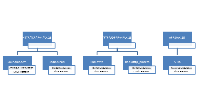
Figure 2 Resulting solutions after hardware decisions
This solution feeds digital data into the radio. And the digital data is generated via the serial port. This solution generates Manchester encoded AX.25 frames encapsulating IPv4 packets.
Radiotftp solution uses tailored software to drive the Radiometrix radio transceivers. The software can run either as a server or as a client depending on its parameters. A client can send WRQ and RRQ requests as stated in TFTP RFC[42]. The TFTP application is built by following the standard OSI layers[52]. The link layer is AX.25. The network layer is UDP/IPv4 [38][35]. These layers ensure that the transmitted data is indeed correct. And the network layer may be used for future work such as routing or forwarding. It is usual for a wireless sensor network to create large amounts of data as time progresses. Therefore an appending option has also been added to the protocol. So the client (i.e. gateway) can send the data as it arrives. The general system diagram can be seen in Figure 3. Below is a list of advantages and disadvantages of this solution.
Advantages:
· This is a tailored solution for the problem, therefore it is reasonable to assume that it will have more performance (i.e. greater throughput).
· It is written completely in C and it is not dependent on Linux kernels, therefore it should be relatively easier to port.
Disadvantages:
· Since it is a tailored solution, it is a less flexible solution (i.e. only file transfer is allowed, command sending or remote shell is not an option).
· Since a serial port is involved, actual AX.25 framing is not an option (AX.25 is a bit based protocol; no bit stuffing, larger MTU, start and stop bits from UART) [33].
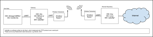
Figure 3. System diagram for radiotftp solution
For the purpose of implementing the project, the C language was chosen for the reasons of portability brought on by extensive use, along with computational efficiency. The methodology of programming was chosen to be event-driven, as this would make porting the program to systems without pre-emption easier than it would with polling type.
The development and deployment platforms were both chosen to be systems based on the Linux kernel due to the flexibility brought on by its open source. However, to retain a wider scope of compatibility and increase the reusability of the code, no libraries that depend on the GNU/Linux system were utilized with the main exception of the portable POSIX functions [59].
The implementation started by implementing each layer of OSI, step by step. First of all the Manchester encoding and decoding utilities have been implemented as the physical layer. After that AX.25 UI message creators and openers have been implemented as Data-link layer. Above that IPv4 packaging functions are implemented as network layer. No routing algorithm other than static routing is implemented, since it would be redundant for our case. But, a useful API is presented to further developers if any routing algorithm is to be implemented. And above all, a programming interface is presented to developers who want to write network applications.
The implementation output was an IP stack built upon and compatible with OSI model standards. This structure is formed only with packaging functions such as package creators or openers. However, the custom API also allows advanced functionality such as packet queues, timer callback assignment and packet reception callback assignment. The workflow of the stack is demonstrated in the pseudocode given in Figure 24.
Network applications often require timer and buffering utilities, so a queuing system and a timer system have been implemented. The queue size was chosen as 1 for this specific implementation as the application requirements dictate that as the maximum queue depth. Similarly, the number of available timers is also set to one as the demand of the TFTP application necessitated only one. However, depending on requirements for other potential uses, the number of timers and the space in transmit queue can be modified. The timers and queue interfaces are abstracted from the rest of the system, allowing their modification to not affect the proper working of the upper layers. The specific details are provided in the header files of the source repository.
Although the software was written to be as independent as possible, some POSIX functions have been used for file operations and timer operations. From the POSIX functions, most frequently used ones are file operations like open, read, write and close. Alarm signal has also been used to set up timers. Furthermore to make the software more operating-system and hardware independent “stdint” library has been used for maximum compatibility among systems[60].
In the end, what software does can be summarized like; the system receives bytes and puts them into a Manchester buffer until a predefined end-of-packet character is received. Then the packet is Manchester decoded, and assuming the packet is an AX.25 UI frame an attempt is made to open it. If successful, the payload of the frame is assumed to be a single UDP/IPv4 packet and is opened. If again successful, then the system routes or multiplexes the packet to the relevant destination or application respectively.
A manual which explains how to configure the radiotftp on both sides have been written during the development. This manual can be used to set up a client and server for wireless sensor network gateways that are using sensd or alikes [61].
This solution feeds digital data into the radio. And the digital data is generated via the serial port. This solution generates Manchester encoded AX.25 frames encapsulating IPv4 packets.
Radiotftp_process solution proposes the use of radiotftp software proposed in solution 1, and porting of this software into Atmega128Rfa1 running Contiki-Os. The radiotftp software will be ported as a Contiki process called radiotftp_process. In this solution the gateway can be completely removed, and the sink mote can personally send the sensor data. This solution is very similar to the solution 1 except for this change. The general system diagram can be seen in Figure 4. Below is a list of predicted advantages and disadvantages of this proposed solution.
Advantages:
· Removal of gateway saves a lot of power (e.g. 5 Watts).
Disadvantages:
· Removal of gateway also means the removal of the gateway storage. So, in a case of broken link or broken receiver, the data is lost instead of being saved in the gateway.
· Requires porting of the software to Atmega128Rfa1 with Contiki, which takes time (even though radiotftp is designed to be portable).
· Since it is a tailored solution, it is a less flexible solution (i.e. only file transfer is allowed, command sending or remote shell is not an option).
· Since a serial port is involved, actual AX.25 framing is not an option (AX.25 is a bit based protocol).
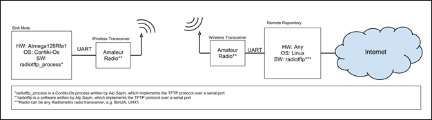
Figure 4 System diagram for radiotftp_process solution
Like in radiotftp solution the of programming was C. This solution was actually a ported and a slightly modified version of the radiotftp software. A Contiki process was written to do exactly the same thing as radiotftp solution does. Contiki processes can be seen analogous to the UNIX pthreads with one major difference. That is, Contiki-OS doesn’t support preemption. So, the Contiki processes have to yield the CPU on their own, allowing other Contiki processes to get their share of the CPU time.
Contiki-OS is a task queuing real time operating system designed specifically for “the internet of things” [3]. Contiki processes work like general purpose operating system tasks, except for the voluntary yielding. Contiki-OS also presents a lot of useful utilities for creating timers, managing memory, using peripherals and most importantly for networking with IP. Since the timers and packet queuing system in radiotftp software was abstracted from the underlying system, it was a rather easy task to modify the relevant parts of the software.
The workflow is as follows: normally, CPU is busy collecting data from environment. But when it is ready to send data, it signals the radiotftp_process and so it wakes up the process. When it wakes up it takes the data from a given pointer as if it is reading a file and transmits it as radiotftp software would send.
UART reception interrupt saves the received byte and treats every byte as Manchester encoded data, but when it receives the predefined end-of-packet character. It copies the received packet into a safe location and wakes the radiotftp_process for processing input data.
In this implementation the lab tests showed that maximum possible baud rate is 4800. It is observed that higher baud rates like 19200 and 38400 require more processing power or a higher CPU frequency.
One disadvantage that this solution brought was the increased level of power saving mode. Normally we can put the CPU into “Power-Down” mode where system clock is halted and a great amount of reduction in power consumption is observed[5]. But with this implementation, due to the necessary enabling of the UART receive interrupt, CPU can be put into “Idle” mode at least[5].
To demonstrate the patching capability of the radiotftp_process to any existing Contiki-OS system with existing processes and resources, a simple Fibonacci Series calculator process is written. Then it’s modified to wirelessly transmit the computed data via radiotftp_process. This process is also a good example to demonstrate how processes and timers work in Contiki-OS.
Finally, the size footprint of the radiotftp_process is also very small. It only adds about five kilobytes to Contiki-Os footprint. The details of the fibonacci application can be found in Figure 5.
|
avr-size --format=berkeley -t fibonacci.avr-atmega128rfa1 text data bss dec hex filename 40809 3506 10052 54367 d45f fibonacci.avr-atmega128rfa1 40809 3506 10052 54367 d45f (TOTALS) Finished building: fibonacci.size
|
Figure 5 Size footprint of Fibonacci application with radiotftp_process
This solution feeds digital data into the radio. And the digital data is generated via the serial port. This solution generates Manchester encoded AX.25 frames encapsulating IPv4 packets. It achieves it by encapsulating the IPv4 packets generated by the kernel and putting them in AX.25 frames. After that the frames are Manchester encoded and sent. Since the packets are generated by the kernel, the transport layer is dependent on the used application (e.g. TFTP uses UDP, while FTP uses TCP). But we decided to use HTTP as mentioned before to take advantage of TCP.
Radiotunnel solution proposes the use of a kernel tunnel interface to create a network kernel interface to drive the Radiometrix transceivers. A software called radiotunnel was written to capture IP packets. Captured IP packets are encapsulated with AX.25 headers. They are Manchester encoded and transmitted through Radiometrix transceivers. The receiver part will capture these frames, decode and unpack them. After that, received IP packets are fed back to the kernel for user programs’ use. The general system diagram can be seen in Figure 6. Below is a list of advantages and disadvantages of this proposed solution.
Advantages:
· Like the soundmodem solution, this is a very flexible solution. It will allow the use of any kind of user programs that use network.
· It’s relatively easy to implement.
Disadvantages:
· As in radiotftp solution, since the underlying hardware will be a serial port, AX.25 will not be fully followed (e.g. no bit stuffing, larger MTU, start and stop bits from UART).
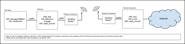
Figure 6 System diagram for radio_tunnel solution
Radiotunnel solution can be viewed as a hybrid of radiotftp solution and soundmodem solution. Like radiotftp it uses the custom AX.25 and IP stacks. It actually makes use of the same codes from radiotftp solution. But unlike radiotftp solution it is library dependent, therefore it is more operating-system dependent. From the runtime point of view, it is more like the soundmodem solution. When you run the solution it creates a network interface in the system. So after set up, it is up to the user to choose what protocol to use to commence the transfers.
The solution is implemented by using user-mode linux utilities [62]. In particular TUN/TAP devices were used [63][64]. TUN/TAP devices are virtual network kernel interfaces, which tunnel the network packets to a software stream. They are easily opened, read, written and closed as if they were files (i.e. POSIX compatible).
TUN devices create IP tunnels, whereas TAP devices create Ethernet tunnels. Since we are not interested in Ethernet in this solution, project proceeded with TUN devices. The newly created interface tunnels the IP packets coming from other applications to a character stream. So, incoming IP packets can be read byte-by-byte from the character stream. And raw IP packets can be written to the same character stream, and they will be received by applications from the interface end.
Basically, a developer can virtualize anything that could be networked to the system. For example a simple ping responder can be seen in Figure 28. In our case the traffic is encapsulated or decapsulated with AX.25 and Manchester protocols, and tunneled into the serial port. The data incoming from serial port is Manchester decoded, and AX.25 unframed, and the payload is directly fed into the TUN device without even checking the content. The data outgoing from the TUN device is first AX.25 framed and then Manchester encoded, and directly fed into the serial port.
But the kernel was assuming that the underlying hardware was full-duplex, and this was a problem for us. Since kernel thought the channel was full-duplex, it wasn’t waiting for the remote side to respond, therefore causing a whole lot of messages to collide and to be dropped. The solution was forcing the radiotunnel to drop some of the packets on the software side. So a rule was hardcoded into the software making sure that, there won’t be any consecutive radio activity within 1 second. This parameter was found to work best by lab testing. Due to the forced packet drops, there was some TCP overhead, but this was found to be the only solution that worked. A further work could implement an actual network interface which can declare the hardware layer as half-duplex. Or a full-duplex radio communication can be used, in that case the forced packet drop wouldn’t be needed.
This solution uses audio ports of a system to generate AFSK modulated signals that carry AX.25 frames. Within the AX.25 frames there can be APRS messages as network/transport layer or IP packets. It achieves it by encapsulating the IPv4 packets generated by the kernel and putting them in AX.25 frames. After that the frames are AFSK modulated and sent. Since the packets are generated by the kernel, the transport layer is dependent on the used application (e.g. TFTP uses UDP, while FTP uses TCP). But as mentioned before we decided to use HTTP
Soundmodem solution uses existing AX.25 kernel headers of Linux and the ‘soundmodem’ software which was written by Thomas Sailor[65][28]. The soundmodem software creates a virtual kernel network interface using the audio ports of a system. After running the software and setting up the hardware connections, two computers can interact with each other as if they are connected via an Ethernet cable. This means any kind of network resource of Linux is available (e.g. TCP/IP). After the setup, a small web server is run to host the incoming data to gateway. Unfortunately, soundmodem software is not yet ready for Bifrost, but it works in a Debian branch called Voyage Linux[14]. For the tests, Voyage Linux has been used. The general system diagram can be seen in Figure 7. Below is a list of advantages and disadvantages of the proposed solution.
Advantages:
· This is a completely standard and a generic solution to the problem, therefore it is more flexible. It even allows running of an http server in the gateway or “ssh”ing into the gateway.
Disadvantages
· It requires more hardware (e.g. volume control circuits, USB audio fobs for Alix boards).
· Initial tests showed that the link is very slow (e.g. 50 bytes/sec) and not so stable (TCP timeout problems).
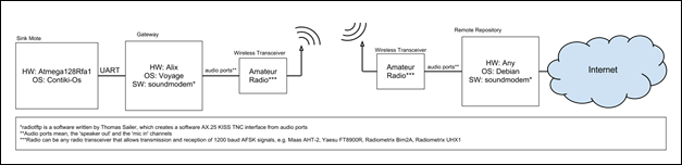
Figure 7 System diagram for soundmodem solution
The soundmodem solution required very less new software writing. But instead, it required custom hardware design such as an audio leveler. Soundmodem software was first set up and tested in a graphical user interface environment such as Ubuntu, where soundmodemconfig utility came in handy for both setup and diagnostics which can be seen in Figures 8 and 11. It was used to configure the soundmodem parameters such as IPv4 settings, channel access settings, delay settings, push-to-talk and sound card settings.
|
|
|
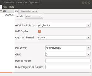
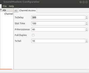
Figure 8 Soundmodemconfig utility configuration options
The aforementioned audio leveler circuit is used to level the audio levels that are going to or coming from the radio. The radio in this solution was either the Maas AHT2-UV or Yaesu FT8900R. The same circuit was also used to control the push-to-talk buttons of the radios. The Maas handheld radio had the PTT controller installed in the microphone port. On the other hand Yaesu station was using a data port to interface any terminal as can be seen in Figure 9.
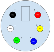
Figure 9 Yaesu FT8900R Data port signals
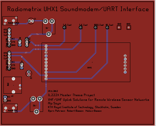
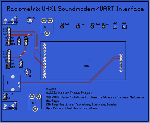
There was no PCB design for this circuitry, since it was a very simple circuit and it was different for Yaesu and the Maas. A card that allows switching between Yaesu and Maas was prepared and used. According to the type of radio that is to be used, the locations of patch cables had to be changed. The schematic of the card can be seen in Figure 12 and the actual can be seen in Figure 10. The details of this card can be found in the soundmodem manual that was written during the development phase [66].
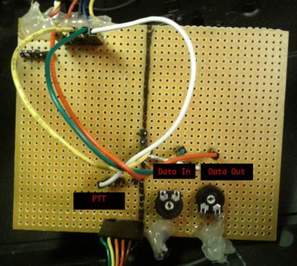
Figure 10 Audio leveler and PTT controller card
|
|
|
|
|
|
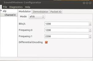
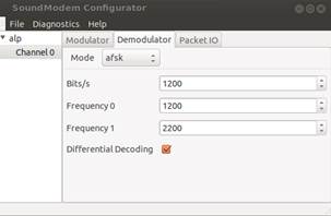
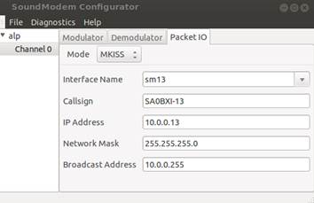
Figure 11 Soundmodemconfig utility channel settings
Then soundmodemconfig’s diagnostic utilities were used to establish and test a link between two computers in lab environment. To test the soundmodem without IP, an AX.25 amateur radio station software called xastir is used [54]. In such, two amateur radio stations were set up and APRS messaging is tested between them. On succession, other utilities that work on IPv4 on AX.25 such as ping, ssh, ftp and wget were used to test the connection. Steps until this were also necessary for the APRS solution, so it should be stated that, it eased the job for perfecting the APRS solution.
What soundmodemconfig does is to create an XML file to be used when soundmodem is invoked. So it is actually possible to configure soundmodem in environments without graphical user interface. So a manual for setting up soundmodem in environments without GUI has been written to ease of future developer or enthusiasts [66].
The next step was to move this solution to Bifrost/ALIX, but unfortunately there were some difficulties with this process. The soundmodem package and some of its required dependencies were not ported to Bifrost. Therefore it was impossible to build or to run the soundmodem utility in Bifrost/Alix. However, a middle way solution was chosen and proceeded with. The Voyage Linux distribution was able to build soundmodem and all of its dependencies [14]. So the final solution requires a Voyage/Alix machine until the soundmodem and its dependencies are ported to Bifrost.
|
|
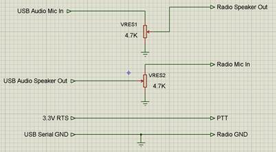
Figure 12 Simple audio leveler and push-to-talk circuit
After setting up the soundmodem, it is possible to have two networked computers. Or, in our case; the gateway and a remote repository computer was networked wirelessly with a half-duplex IPv4 link. Then the project proceeded with setting up an Apache web server on the gateway side, and using wget or similar on the client side to fetch the collected data.
This solution uses APRS as application, network and transport layer. The measurement data is converted into APRS telemetry messages and transmitted.
Aprs solution proposes the transmission of collected data to the APRS network. This solution requires the soundmodem software and aprx software running as beacon. When the data arrives from the WSN, a small bash script converts this data into an APRS telemetry message and transmits it into air. If there are any APRS listeners, they will pick-up and probably forward this message to the APRS database. For testing this solution, an APRS I-Gate (i.e. RF-to-internet forwarder) will also be set up. The general system diagram can be seen in Figure 13. Below is a predicted list of advantages and disadvantages of this proposed solution.
Advantages:
· This is a completely standard solution.
· This solution can utilize the existing APRS network if there are any.
Disadvantages:
· APRS restrictions may cause data loss, or there may not be enough space for our data (e.g. minimum time between consecutive APRS transmissions, APRS telemetry allows 5 types of data only).
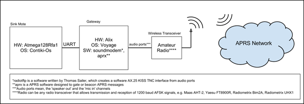
Figure 13 System diagram for APRS solution
APRS solution is implemented by again setting up the soundmodem software and hardware. But instead of IP, APRS is used as the transport layer. And for that purpose the aprx software is used. Aprx is a simple command line, amateur radio station software which is generally used for Rx-to-Inet, Inet-to-Tx, and Rx-to-Tx digipeating purposes. It also has features like periodically transmitting APRS messages or sending automated traffic statistics. It is simply configured by editing an aprx.conf file whose can be seen below in Figure 14.
|
mycall SA0BXI-13 #mycall must be the same port in axports file
<aprsis> server rotate.aprs2.net </aprsis>
<logging> pidfile /var/run/aprx.pid rflog /var/log/aprx/aprx-rf.log aprxlog /var/log/aprx/aprx.log </logging>
<interface> ax25-device $mycall tx-ok true </interface>
<beacon> beaconmode both cycle-size 20m beacon symbol "R&" lat "6016.35N" lon "02506.36E" comment "Rx-only iGate" beacon file /tmp/wxbeacon.txt </beacon> |
Figure 14 Simple configuration file for aprx,
As mentioned before, APRS telemetry messaging was found to fit best for our purposes. Simply explained, APRS telemetry messages support transmission and logging of five analog values and eight binary values. User has to send four different kinds of messages to properly transmit telemetry data. These are label, data, coefficient and project name messages. From these four only label, data and coefficient messages are necessary. Also, label and coefficient messages can be transmitted less frequent then data messages.
Unfortunately aprx does not provide any telemetry utilities. But it has an option for transmitting custom raw APRS messages that are stored in a text file. This option is called the beaconing. Beaconing has several options. Aprx does not specifically watch the file for changes, but instead a time interval is set up and the APRS messages in the text file are sent periodically according to the setting in aprx.conf. So a shell script can be written to change the designated beacon file.
One issue with aprx software was the built-in automated telemetry messages. Aprx is hard-coded to send telemetry messages about the station’s usage and traffic statistics. This was causing a problem since the telemetry information was colliding and therefore the resulting data was being corrupted. To fix this issue, aprx source has been tampered with to disable this automated telemetry messages. This simple fix can be found in Figure 30.
In the end all that is left for the user is to set up a shell script and aprx settings to set up the whole system. Finally, to save the user from the details of APRS protocol, a simple command line utility called aprs_telemetrit is written (Figure 15). This utility simply takes in the telemetry message parameters as program arguments and outputs the raw telemetry message. So, all the user has to do is to set up a simple shell script like in Figure 30.
|
telemetrit type callsign receiver_callsign [content] type = data,label,unit,coef,bitsense
example for data: telemetrit data NOCALL NOCALL-1 sequence_number A1 A2 A3 A4 A5 B1 B2 B3 B4 B5 B6 B7 B8 unwanted telemetry data can be omitted starting from the left
example for label: telemetrit label NOCALL NOCALL-1 A1 A2 A3 A4 A5 B1 B2 B3 B4 B5 B6 B7 B8 unwanted labels can be omitted starting from the left
example for unit: telemetrit unit NOCALL NOCALL-1 A1 A2 A3 A4 A5 B1 B2 B3 B4 B5 B6 B7 B8 unwanted units can be omitted starting from the left
example for coef: telemetrit coef NOCALL NOCALL-1 A1a A1b A1c A2a A2b A3a A3b A3c A4a A4b A4c A5a A5b A5c unwanted coefficients can be omitted starting from the left, they'll be set to 0
example for bitsense: telemetrit bitsens NOCALL NOCALL-1 project_name B1 B2 B3 B4 B5 B6 B7 B8 unwanted coefficients can be omitted starting from the right, they'll be set to 0 Build Date: Sep 3 2012 12:37:03 |
Figure 15 aprs_telemetrit usage
Within this project, four different sets of experiments have been conducted. Design of the experimentation phase was made according to the initial lab tests. The aim in this design was to minimize the required time and was to emphasize the difference between solutions. The initial experiment plan was to have three sets of experiments in three days; first day with 433 MHz band, second day with 144 MHz band, and finally third day with both bands in lab environment.
Due to an antenna mismatch problem, these experiments had to be canceled and the data collected in first day had to be ignored. After this incident, and after the antenna mismatch problem has been solved, a more thorough experiment is created and executed. The plan was to first have an initial set of non-lab experiments with all bands and equipment to verify the hardware and software, and to detect and fix if any errors/problems to be found. This test is conducted in Kista with a maximum clear line-of-sight of about 650 meters. Although some data was collected in these tests, they were only used to optimize the software and hardware for the latter experiments. After the Kista testing a little optimization is made to software, decreasing the MTU of transmitted packets, therefore decreasing the probability of a packet drop due to noise.
After this verification stage, the initial plan is revised and executed. The details of this plan are as below. All experiments have been done in an open field with clear line of sight. Some of the experiments below are marked as optional, which means they will be performed only if the time allows. Else they were to be put under the title of further work.
These experiments will cover the radiotftp and radiotftp_process solutions. For testing, two Ubuntu laptops will be set up to use radiotftp to transfer files. Builtin data logger of radiotftp will be used to collect the below stated data. No experiments will be done with radiotftp_process, since their base codes –therefore the protocol stacks and timings- are the same. Transfer sizes are chosen as single and 16 packets to observe the differences between single packet and many-packet transfers. Since we are using amateur radio bands, we are actually not allowed to use ~100% channel utilization, but in the name of science we will test it. In the application notes for Radiometrix devices, it is said that lower baud rates have a direct impact on the range. Therefore we are going to use fixed average baud rates. The transmission power will be fixed to 10 mW (10 dBm). The VHF frequency to be used is 433.925 Mhz, and UHF frequency to be used will be decided in field (which will be between 144 and 146 MHz). And finally, for the sake of simplicity transfers will be declared as disconnected, after a certain amount of consecutive retransmissions. For our experiments, this amount is designated as 8. This number is chosen through several lab tests to ensure temporal noises do not cause disconnections. Measurements will be done four times and will be averaged for increased accuracy. They will be performed separately for Bim2A and UHX1.
Parameters:
1. Distance
2. Transfer Size
Input Range:
1. Distance = [2m:2km] (7 points)
2. Transfer Size = [127 bytes, 16*128 bytes],
Outputs:
1. Transfer Time
2. Throughput
3. Packet Error Rate
4. Energy consumption
5. Power consumption
-Throughput will be derived from transfer time.
-Packet error rate will be derived from number of retransmissions.
-Energy consumption will be derived from datasheet data and amount of Tx enabled/disabled time.
-Power consumption will be derived from energy consumption by differentiating over transfer time.
These experiments will cover the radio_tunnel and soundmodem solutions. Below explained measurements will be done with radio_tunnel and soundmodem separately. For radio_tunnel baud rates will be fixed to 19200 for Bim2A and 2400 for UHX1. For soundmodem the bitrate is already fixed to 1200 bps due to the usage of AFSK. The transfer sizes are chosen as 127 bytes and 2 kbytes to observe the difference between single packet and many packet transactions (MTU is 255 bytes). The transmission power will be fixed to 10 mW (10 dBm). The VHF frequency to be used is 433.925 Mhz, and UHF frequency to be used will be decided in field (which will be between 144 and 146 MHz). Measurements will be done four times to increase accuracy.
Parameters:
1. Transfer Size
Input Range:
1. Transfer Size = [127 bytes, 2048 bytes]
Outputs:
1. Transfer time
2. Throughput
3. Instantaneous Channel Utilization
4. Average Channel Utilization
5. Energy Consumption
6. Power Consumption
-Throughput will be derived from transfer time.
-Energy consumption will be derived from datasheet data and amount of Tx enabled/disabled time
-Power consumption will be derived from energy consumption by differentiating over transfer time
-Instantaneous channel utilization will be derived from measuring the Tx enabled/disabled time
-Average channel utilization will be derived from instantaneous channel utilization by integrating over transfer time.
Without the use of any software, the performances of Bim2A and UHX1 will be measured. To do this, the carrier signal will carry no information but a complete set of zeros (grounded Tx). On the receiver side, RSSI output of the radiometrix devices will be measured. Later on, this data can be used to map RSSI level to the performance data obtained in first two experiments.
Parameters:
1. Distance
Input Range:
1. Distance = [2m:2km] (7 points)
Outputs:
1. Rssi Voltage
2. Rssi
-Only the signal strength will be tested in the experiment.
-Rssi will be derived from using the RSSI voltage data by mapping it with the plots provided in datasheet (if provided).
Without the use of any software, the performance of UHX1 will be measured. To do this, the carrier signal will carry no information but a complete set of zeros (grounded Tx). On the receiver side, RSSI output of the Radiometrix devices will be measured. Later on, this data can be used to map Tx Power level to the performance data obtained in first three experiments.
Parameters:
1. Distance
2. Tx Power (dBm)
Input Range:
1. Distance = [2m:inf*] (16 points)
2. Tx Power = [10:1:30] (10 to 30 dBm with 1 dBm steps)
-Only the signal strength will be tested in this experiment.
-Rssi will be derived from using the RSSI voltage data and mapping it with the plots provided in datasheet.
-Distance will be increased exponentially.
*inf means until the connection is lost, which means rssi is less than or equal to the carrier detect level.
As the experiment area, Riddarholmen in Gamla Stan is chosen. This location was able to provide a maximum a 2.1 kilometers of clear line-of-sight without even the interruption of Fresnel zones. The experiment map can be seen below in Figure 16. The marked location zero is the fixed base station, and the other locations are the mobile station test points. A file transfer was made several times with different parameters from points 1-7 to 0. Mobile station sent the designated files to the fixed station. Note that during the transfers the mobile station was also fixed. The positions were saved by using the built-in GPS in a Nokia E5-00 mobile phone.
|
Test Point |
Distance to Base Station (±10 meters) |
|
1 |
395 meters |
|
2 |
700 meters |
|
3 |
1050 meters |
|
4 |
1390 meters |
|
5 |
1820 meters |
|
6 |
1950 meters |
|
7 |
2120 meters |
Table 1 Distances of test points to base station in Riddarholmen
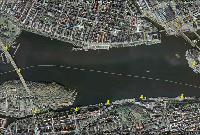
Figure 16 Map of Gamla Stan Experiments
In the open field only radiotftp was tested due to the time requirement and also due to the immobility of the other solutions. Radiotftp solution was tested with both bands trying find out the average transfer time, average packet drop percentage and maximum distance that Radiometrix devices can reach with a fixed power (10 milliwatts in our case). Radiotftp_solution was not included in experiments since the protocol and the hardware it used was the same with Radiotftp, but it was verified to be working. Radiotunnel and Soundmodem were only tested in lab environment, since they required much more time for a transfer relative to the radiotftp. And finally APRS solution was tested only by sending out some sample telemetry data with aprx software.
The radiotunnel and radiotftp software was modified to log events such as, TX/RX switching, packet drop, packet transmission, request reception and error transmission and error reception. The sample of such event log can be seen in Table 4 and the format can be seen in Table 5 in Appendix C. For other solutions UNIX time facilities were used for time measurement [67]. After the data collection, a utility was written to facilitate parsing of data logs and generation of plots and tables [68].
After collecting the data a lot of time was spent to plot them into meaningful numbers and statistics. Depending on the point of view we have gathered a lot of interesting data. Below are the discussions regarding these data. Note that all raw data is currently accessible in the author’s home page [69].
Below are the plots and tables that summarize some key measurements of these experiments with radiotftp solution and general experiments with other solutions. The disconnected cases are discarded from the plots, therefore fewer samples can be observed in some of these plots. In any case these plots also explain some important points about 144 and 434 Mhz bands irrelevant to the protocol that is used.
|
Transfer Time 127 bytes |
Transfer Time 2 kbytes |
|
|
radiotftp uhx1 |
00:08.915 |
00:21.727 |
|
radiotftp bim2a |
00:00.873 |
00:02.414 |
|
radiotunnel uhx1 |
02:56.029 |
12:09.429 |
|
radiotunnel bim2a |
02:00.120 |
02:05.261 |
|
soundmodem |
02:09.707 |
02:59.324 |
Table 2 Average transfer times with minimum distance between transceivers
|
Figure 17 Transfer time plots for single packet delivery |
Figure 18 Transfer time plots for many-packet delivery |
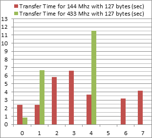
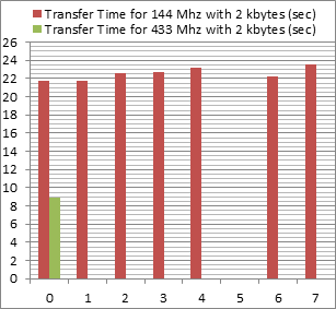
In 434 Mhz experiments which are performed with Bim2a, it can be observed that in 2 kbytes experiments almost all trials went into disconnection, even from the first location with distance of 400 meters (Figures 20 & 21). Therefore we can say that, if multi-packet transactions are going to be performed with 434 Mhz band, a greater consecutive retransmit limit is required (more than 8). On the other hand, when we consider the ideal conditions case -1 meter distance-, multi-packet transactions are better to avoid the effects of overhead and it gives more bitrate (Figures 18,19 & 22,23).
|
Figure 19 Error rate plots for single packet delivery |
Figure 20 Error rate plots for many-packet delivery |
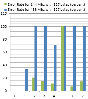
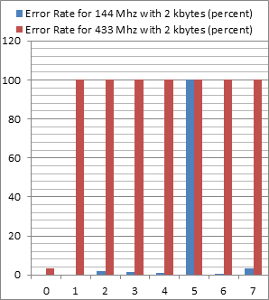
In 434 Mhz band, the results of 127 byte experiments point to one important conclusion. With distance, the error rate increases a lot (Figures 20 & 22). And after about 400 meters, the error rate becomes too much that it impossible to transfer files. And even with 400 meters distance, the error rate is too high that, 144 Mhz band has lower transfer times compared to 434 Mhz band (even with the higher baud rate advantage). The other important point is that we observe connection with about 1400 meters distance. That is the location 4 with higher ground with respect to others. We see that effect of higher ground helps overcome the distance effect. But as can be seen from Figure 19 Error rate plots for single packet delivery the error rate is just too high to be feasible enough for actual use. The 2 kbytes experiments also support this with disconnection in all tests from the same location.
|
Figure 21 Bitrate plots for single packet delivery |
Figure 22 Bitrate plots for many-packet delivery |
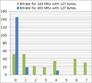
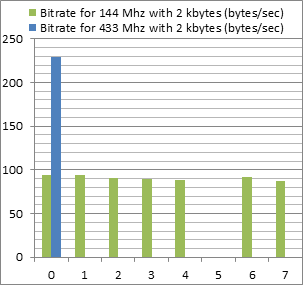
In 144 Mhz experiments which are performed with Uhx1, first thing to observe is the existence of a connection even from 2100 meters with a low error rate of about 3.5 percent. Other thing that we observe is; error rate does not change too much with respect to distance. This also brings a stable transfer time and bitrate with respect to distance. These observations tell that the fade margin of the UHX1s is better than Bim2As (see the fall in RSSI and increase in error rate of both devices, Table 3, Figure 19 Error rate plots for single packet delivery and Figure 20 Error rate plots for many-packet delivery. The effect of single-packet transactions can also be observed in 144 MHz experiments, adding overhead delay.
Finally, there is one last important point about all radiotftp experiments. The fifth location which is about 1820 has no values in any of the plots. That’s because there was actually an obstruction in the signal path. Although the obstruction was observable, the experiments continued also at this point to observe the effect of obstructions. This obstruction in our case was some woods, which can also be observed in the map in Figure 16. The effect of this obstruction was complete loss of signal in both bands.
The fourth location with a distance of about 1400 meters was also different from others; it was higher than the others. The increase in RSSI and drop in error rates in fourth location can be tied to this cause.
These observations emphasize the importance of one thing, which is the importance of having a clear line-of-sight, which may be obtained by having a high ground.
|
Location |
RSSI (UHX1) |
RSSI (Bim2a) |
|
No Signal Applied |
64 |
0.28 |
|
0 (Base) |
196 |
0.48 |
|
1 |
136 |
0.40 |
|
2 |
122 |
0.30 |
|
3 |
116 |
0.31 |
|
4 |
133 |
0.38 |
|
5 |
103 |
N/A |
|
6 |
126 |
N/A |
|
7 |
121 |
N/A |
Table 3 RSSI readings from various locations with UHX1 and Bim2A
Regarding the whole project we can say that it was a successful project, and it is indeed possible to use VHF/UHF bands for wireless sensor network uplinks with more than one different implementations for a relatively low financial cost. It was also interesting to explore different bands and/or protocols and their effects. For example; the increase in throughput and the decrease in range with the use of higher frequency were interesting. The Contiki integration is also an interesting outcome of the project due to the removal of the gateway from the process. As for the project goals, the project has successfully reached its goals to implement a feasible IP link with less than 100 mW transmit power which can reach over 2km with only 10 mW transmit power.
Apart from these general points, important conclusions that are obtained from the experiments are as below. After the collection of data, via various utilities the raw data have been parsed and processed. Although many of the results were expected, there were also few which were unexpected.
Concerning only radiotftp:
· The effect of overhead can be heavily observed. On the other hand, many-packet transactions are statistically more probable to disconnect (‘Experiments with radiotftp’).
· The bitrate difference in bands shows itself also in the final throughput.
· While using the 2 meter band, the distance does not seem to have much effect. On the other hand, obstructions on the wave path cause a lot of distortion.
· While using the 70 cm band, the received power decays much more relative to the 2 meter band and therefore observed to have a much shorter range.
· In both bands having a high ground has a good impact on signal strength.
Concerning all solutions together:
· Radiotftp solution seems to have much greater bitrate compared to others, but this is simply an effect of utilizing the channel more efficiently. On the other hand, other solutions can’t use the channel this efficiently, even if they wanted to.
· The radiotunnel solution shows almost an exponential growth in transfer time with respect to the file size. This is due to the manual forced drop of the packets to ensure half-duplex operation.
· Soundmodem proved itself to be a faster option compared to radiotunnel, even with its low raw bitrate (1200 bps).
· If the radiotunnel is not to be improved to act as an half-duplex interface, and if soundmodem solution can be improved to use radiometrix devices, then radiotunnel solution can deprecated.
· Some suggestions could be made according to some requirements:
o If higher throughput is required; radiotftp,
o If easy-setup and easy API is required; radiotunnel
o If standardization and easy API is required; soundmodem
o If standardization and set-it-and-forget-it kind of application is required; APRS solution would be suggested.
As can be observed, each solution addresses a specific requirement. Therefore there is not one `best` solution in this project.
Below are some points that, future developers and researchers should consider. These are not only suggestions, but also guidelines for further development.
Radiotftp
· The radiotftp code base should be improved to have multiple-size queues and multiple timers. It already supports it, but it is not a default.
· The radiotftp code should be cleaner for further developers. It should look like an open API -which, it is-, and there should be an open documentation for it.
· The radiotftp solution can be optimized more by changing the place of the delays and/or replacing the delays with non-busy waits.
Radiotftp_process
· The radiotftp_process code could be optimized to work with higher baudrates than 2400. So that it would consume less CPU time while transmission.
Radiotunnel
· The radiotunnel code should not be improved anymore, but instead, an actual device driver should be written for fine tuning.
Soundmodem
· The soundmodem solution should be moved on to work with Radiometrix devices. In such way, a more portable hardware can be obtained. And the users won’t need to worry about handheld radios’ power consumption.
APRS
· If possible, the APRS solution should also be tested in open field and packet loss should be recorded.
Others
· The uhx1_programmer can be extended to be able to program the frequency of the UHX1 devices, so that frequency can be selected while running to avoid interference [70].
· The devtag library could be incorporated to use USB device tags instead of USB device names to select the proper USB FTDI device [71].
· A team has already started working on an implementation of a Delay Tolerant Network (DTN) based on this project’s outcomes [18].
[1] Robert Olsson, ‘Herjulf Mote’. [Online]. Available: http://herjulf.se/products/WSN/sensors/General-Description-v1.4.txt. [Accessed: 08-February-2013].
[2] ‘IEEE 802.15.4’. [Online]. Available: http://www.ieee802.org/15/pub/TG4.html. [Accessed: 21-February-2012].
[3] ‘The Contiki OS’. [Online]. Available: http://www.contiki-os.org/. [Accessed: 29-February-2012].
[4] ‘Wireless Sensor Network Topologies | Sensors’. [Online]. Available: http://www.sensorsmag.com/networking-communications/wireless-sensor-network-topologies-778. [Accessed: 08-February-2013].
[5] ‘ATmega128RFA1- Atmel Corporation’. [Online]. Available: http://www.atmel.com/devices/ATMEGA128RFA1.aspx. [Accessed: 21-February-2012].
[6] ‘IL2213 WSN-Projects Fall 2011’. [Online]. Available: http://www.tslab.ssvl.kth.se/csd/files/wsn/index.html. [Accessed: 21-February-2012].
[7] Prodromos Mekikis, Guodong Guo, Stefano Vignati, Saad Fakher, Ibrahim Kazi, and Mussie Tesfaye, ‘Contiki-OS on Atmega128RFA1’. KTH, 20111212, Available at http://www.tslab.ssvl.kth.se/csd/files/wsn/contiki-final-report.pdf.
[8] Alp Sayin, Angeline Thiruthuvadoss, Hesham Omran, Junzhe Tian, Rui Li, and Yihui Wang, ‘TinyOS on Atmega128RFA1’. KTH, 20111213, Available at http://www.tslab.ssvl.kth.se/csd/files/wsn/tinyos-final-report.pdf.
[9] P. Levis, ‘TinyOS Programming’. 20061027, Available at http://www.tinyos.net/tinyos-2.x/doc/pdf/tinyos-programming.pdf.
[10] D. Gay, P. Levis, D. Culler, and E. Brewer, ‘nesC 1.1 Language Reference Manual’. 20030501, Available at http://nescc.sourceforge.net/papers/nesc-ref.pdf.
[11] A. Dunkels, F. Österlind, and Z. He, ‘An adaptive communication architecture for wireless sensor networks’, 2007, p. 335, DOI:10.1145/1322263.1322295, Available at http://portal.acm.org/citation.cfm?doid=1322263.1322295.
[12] ‘PC Engines alix2d13 product file’. [Online]. Available: http://pcengines.ch/alix2d13.htm. [Accessed: 21-February-2012].
[13] ‘Bifrost/Linux resources’. [Online]. Available: http://bifrost.slu.se/. [Accessed: 21-February-2012].
[14] ‘Voyage Linux | { x86 Embedded Linux = Green computing }’. [Online]. Available: http://linux.voyage.hk/. [Accessed: 24-May-2012].
[15] ‘Raspberry Pi | An ARM GNU/Linux box for $25. Take a byte!’ [Online]. Available: http://www.raspberrypi.org/. [Accessed: 08-February-2013].
[16] ‘Debian -- ARM Port’. [Online]. Available: http://www.debian.org/ports/arm/. [Accessed: 08-February-2013].
[17] R. Olsson and J. Laas, Sensd. 20120610, Available at https://github.com/herjulf/sensd.
[18] Technology Transfer Alliance, ‘Technology Transfer Alliance WSN Team Fall 2012’, Technology Transfer Alliance WSN Team Fall 2012. [Online]. Available: http://ttaportal.org/menu/projects/wsn/fall-2012/.
[19] G. Werner-Allen, K. Lorincz, M. Ruiz, O. Marcillo, J. Johnson, J. Lees, and M. Welsh, ‘Deploying a wireless sensor network on an active volcano’, Internet Computing, IEEE, vol. 10, no. 2, pp. 18 – 25, April 2006, DOI:10.1109/MIC.2006.26.
[20] G. Werner-Allen, J. Johnson, M. Ruiz, J. Lees, and M. Welsh, ‘Monitoring volcanic eruptions with a wireless sensor network’, in Wireless Sensor Networks, 2005. Proceeedings of the Second European Workshop on, 2005, pp. 108 – 120, DOI:10.1109/EWSN.2005.1462003.
[21] ‘Ranger : FreeWave Technologies’. [Online]. Available: http://www.freewave.com/products/allproducts/rangerseries.aspx. [Accessed: 25-May-2012].
[22] A. Mainwaring, D. Culler, J. Polastre, R. Szewczyk, and J. Anderson, ‘Wireless sensor networks for habitat monitoring’, 2002, p. 88, DOI:10.1145/570738.570751, Available at http://portal.acm.org/citation.cfm?doid=570738.570751.
[23] T. L. Dinh, W. Hu, P. Sikka, P. Corke, L. Overs, and S. Brosnan, ‘Design and Deployment of a Remote Robust Sensor Network: Experiences from an Outdoor Water Quality Monitoring Network’, 2007, pp. 799–806, DOI:10.1109/LCN.2007.39, Available at http://ieeexplore.ieee.org/lpdocs/epic03/wrapper.htm?arnumber=4367918.
[24] T. Naumowicz, R. Freeman, H. Kirk, B. Dean, M. Calsyn, A. Liers, A. Braendle, T. Guilford, and J. Schiller, ‘Wireless Sensor Network for habitat monitoring on Skomer Island’, in Local Computer Networks (LCN), 2010 IEEE 35th Conference on, 2010, pp. 882 –889, DOI:10.1109/LCN.2010.5735827.
[25] ‘Part 97 - Amateur Radio’. [Online]. Available: http://www.arrl.org/part-97-amateur-radio. [Accessed: 24-May-2012].
[26] ‘Definition: manchester code’. [Online]. Available: http://www.its.bldrdoc.gov/fs-1037/dir-022/_3206.htm. [Accessed: 25-May-2012].
[27] A. Telephone and T. Company, Data sets 202S and 202T interface specification. The Company, 1976, Available at http://books.google.se/books?id=OX7zGgAACAAJ.
[28] ‘Multiplatform Soundcard Packet Radio Modem Driver Software’. [Online]. Available: http://www.baycom.org/~tom/ham/soundmodem/. [Accessed: 25-May-2012].
[29] ‘Radiometrix - Radio Modules - RF Modules - Wireless Modules | BiM2A’. [Online]. Available: http://www.radiometrix.com/content/bim2a. [Accessed: 21-February-2012].
[30] ‘Radiometrix - Radio Modules - RF Modules - Wireless Modules | UHX1’. [Online]. Available: http://www.radiometrix.com/node/184. [Accessed: 25-May-2012].
[31] ‘Radiometrix - Error Performance of BIM Transceiver with RS232 Interface’. [Online]. Available: http://www.rfmodules.com.au/rm/apps/apnt101.htm. [Accessed: 17-February-2013].
[32] ‘Ethernet Technologies - DocWiki’. [Online]. Available: http://docwiki.cisco.com/wiki/Ethernet_Technologies. [Accessed: 25-May-2012].
[33] William A. Beech, Douglas E. Nielsen, and Jack Taylor, ‘AX.25 Link Access Protocol for Amateur Packet Radio’. Available at http://www.tapr.org/pdf/AX25.2.2.pdf.
[34] Information Sciences Institute University of Southern California, ‘INTERNET PROTOCOL’. September-1981, Available at http://www.ietf.org/rfc/rfc791.txt.
[35] IETF, ‘Internet Protocol, Version 6 (IPv6) Specification’. [Online]. Available: http://www.ietf.org/rfc/rfc2460.txt. [Accessed: 25-May-2012].
[36] APRS Working Group, ‘APRS Protocol Reference Version 1.0’. Tucson Amateur Radio Corp, 2000, Available at http://www.aprs.org/doc/APRS101.PDF.
[37] ‘Google Maps APRS’. [Online]. Available: http://aprs.fi/. [Accessed: 25-May-2012].
[38] ‘User Datagram Protocol’. [Online]. Available: http://www.ietf.org/rfc/rfc768.txt. [Accessed: 26-May-2012].
[39] ‘RFC 793 - Transmission Control Protocol’. [Online]. Available: http://tools.ietf.org/html/rfc793. [Accessed: 04-February-2013].
[40] J. Postel and J. Reynolds, ‘File Transfer Protocol (FTP)’, 19851001. [Online]. Available: http://www.ietf.org/rfc/rfc959.txt. [Accessed: 08-February-2013].
[41] IETF Network Working Group, ‘Hypertext Transfer Protocol -- HTTP/1.1’. Available at http://www.ietf.org/rfc/rfc2616.txt.
[42] ‘THE TFTP PROTOCOL (REVISION 2)’. [Online]. Available: http://www.ietf.org/rfc/rfc1350.txt. [Accessed: 26-May-2012].
[43] M. Krasnyansky and M. Yevmenkin, ‘Universal TUN/TAP device driver’. [Online]. Available: http://www.kernel.org/doc/Documentation/networking/tuntap.txt. [Accessed: 25-May-2012].
[44] ‘Digipeater - APRSWiki’. [Online]. Available: http://info.aprs.net/index.php?title=Digipeater. [Accessed: 29-February-2012].
[45] Alan Crosswell, ‘APRS from the Bottom Up’. 20021230, Available at http://www.users.cloud9.net/~alan/ham/aprs/aprs.pdf.
[46] ‘draft-ietf-core-coap-12’. [Online]. Available: https://datatracker.ietf.org/doc/draft-ietf-core-coap/. [Accessed: 15-October-2012].
[47] L. Richardson, RESTful web services. Farnham: O’Reilly, 2007, ISBN: 9780596529260.
[48] M. Kovatsch, S. Duquennoy, and A. Dunkels, ‘A Low-Power CoAP for Contiki’, in Mobile Adhoc and Sensor Systems (MASS), 2011 IEEE 8th International Conference on, 2011, pp. 855 –860, DOI:10.1109/MASS.2011.100.
[49] International Organization for Standardization, International Electrotechnical Commission, and Institute of Electrical and Electronics Engineers, Information technology telecommunications and information exchange between systems-- local and metropolitan area networks-- specific requirements. Part 11, Wireless LAN medium access control (MAC) and physical layer (PHY) specifications = Technologies de l’information : télécommunications et échange d’information entre systèmes-- réseaux locaux et métropolitains-- exigences spécifiques. Partie 11, Spécifications du contrôle d’accès du milieu sans fil (MAC) et de la couche physique (PHY). Geneva; New York: ISO : IEC ; Institute of Electrical and Electronics Engineers, 2012, ISBN: 9780738180076 0738180076, Available at http://ieeexplore.ieee.org/servlet/opac?punumber=6361246.
[50] ‘MAAS-AHT-2-UV-Handfunkgeraet-VHF-UHF’. [Online]. Available: http://maas-elektronik.de/MAAS-AHT-2-UV-Handfunkgeraet-VHF-UHF.2.html. [Accessed: 25-May-2012].
[51] ‘YAESU FT-8900R’. [Online]. Available: http://www.yaesu.com/indexvs.cfm?cmd=DisplayProducts&ProdCatID=106&encProdID=0C4855ADE6394D514EAABAE148B93F5C&DivisionID=65&isArchived=0. [Accessed: 25-May-2012].
[52] ‘The OSI Model’s Seven Layers Defined and Functions Explained’. [Online]. Available: http://support.microsoft.com/kb/103884. [Accessed: 29-February-2012].
[53] ‘Aprx.en – HamFi’. [Online]. Available: http://wiki.ham.fi/Aprx.en#Installation. [Accessed: 25-May-2012].
[54] The Xastir Group, ‘XastirWiki’. [Online]. Available: http://www.xastir.org/wiki/Main_Page.
[55] Apache Foundation, Apache Http Server Project. Available at http://httpd.apache.org/.
[56] GNU GPL, GNU Wget. Available at http://www.gnu.org/software/wget/.
[57] T. Ylonen and S. Lehtinen, ‘SSH File Transfer Protocol’, 20011001. [Online]. Available: http://filezilla-project.org/specs/draft-ietf-secsh-filexfer-02.txt. [Accessed: 08-February-2013].
[58] Future Technology Devices International Limited (FTDI), ‘TTL to USB Serial Converter Range of Cables Datasheet’. 20100902, Available at http://www.ftdichip.com/Support/Documents/DataSheets/Cables/DS_TTL-232R_CABLES.pdf.
[59] IEEE, ‘POSIX IEEE Std 1003.1TM-2008’. Available at http://pubs.opengroup.org/onlinepubs/9699919799/.
[60] IEEE, ‘stdint.h - integer types’. Available at http://pubs.opengroup.org/onlinepubs/007904975/basedefs/stdint.h.html.
[61] Alp Sayin, ‘Manual for Setting up Radiotftp’. Available at http://alpsayin.com/master_thesis/docs/Manual%20for%20Setting%20Up%20Radiotftp.pdf, [accessed August 28, 2012].
[62] ‘The User-mode Linux Kernel Home Page’. [Online]. Available: http://user-mode-linux.sourceforge.net/old/. [Accessed: 29-August-2012].
[63] ‘Universal TUN/TAP driver - FAQ’. [Online]. Available: http://vtun.sourceforge.net/tun/faq.html. [Accessed: 25-May-2012].
[64] ‘Setting up the network’, User Mode Linux. [Online]. Available: http://user-mode-linux.sourceforge.net/old/networking.html. [Accessed: 29-August-2012].
[65] ‘LinuxHam’. [Online]. Available: http://www.linux-ax25.org/wiki/Main_Page. [Accessed: 26-May-2012].
[66] Alp Sayin, ‘Manual for Setting up Soundmodem’. Available at http://alpsayin.com/master_thesis/docs/Manual%20for%20Setting%20Up%20Soundmodem.pdf.
[67] ‘time(2) - Linux man page’, time(2) - Linux man page, 20121709. [Online]. Available: http://linux.die.net/man/2/time.
[68] ‘radio-event-reader’, GitHub. [Online]. Available: https://github.com/alpsayin/radio-event-reader. [Accessed: 29-September-2012].
[69] Alp Sayin, ‘Experiment Data for VHF/UHF Wireless Uplink Solutions for Remote Wireless Sensor Networks’. [Online]. Available: http://alpsayin.com/master_thesis/data/. [Accessed: 08-February-2013].
[70] WSN Team 2012, Radio-Daemon. Available at https://github.com/WSN-2012/Radio-Daemon, [accessed November 28, 2012].
[71] J. Låås, devtag. Available at https://github.com/jelaas/devtag, [accessed November 28, 2012].
Master Thesis Webpage:
http://alpsayin.com/vhf_uhf_uplink_solutions_for_remote_wireless_sensor_networks
Radiotftp Source:
https://github.com/alpsayin/radiotftp
Modified Sensd Source:
https://github.com/alpsayin/sensd
Original Sensd Source:
https://github.com/herjulf/sensd
Radiotftp_process Source:
https://github.com/alpsayin/radiotftp_process
Radiotunnel Source:
https://github.com/alpsayin/radiotunnel
APRS Telemetrit Source:
https://github.com/alpsayin/aprs_telemetrit
UHX1 R/N Calculator Source:
https://github.com/alpsayin/uhx1_rn_calculator
UHX1 Programmer Source:
https://github.com/alpsayin/uhx1_programmer
UHX1 Board PCB Design Source:
https://github.com/alpsayin/uhx1_uart_pcb
Bim2A Board PCB Design Source:
https://github.com/alpsayin/bim2a_uart_pcb
Radio Event Reader Source:
https://github.com/alpsayin/radio-event-reader
Old Software Repository in Google Code:
http://code.google.com/p/kth-wsn-longrange-radio-uplink/
TinyOS Port for Atmega128Rfa1 Source:
http://code.google.com/p/kth-wsn-atmega128rfa1-tinyos/
|
Uart_interrupt_handler() { RaiseFlag() SaveReceivedByte() } Main() { While(1) { //…other tasks performTasks()
If( Byte_received ) { putByteIntoManchesterBuffer(newByte) if( newByte is END_OF_PACKET) { openManchesterPacketIntoAX25Buffer(&src, &dst, &content) if( validPacket ) { openUDPIPv4Packet(&src, &dst, &src_port, &dst_port, &content) if( validPacket ) { udpPacketMultiplexer(src,dst,srcport,dstport,content) } } }
//…other tasks performTasks()
If( aPacketIsPendingToBeSent ) { If( notInTheMiddleOfReception ) { TransmitNextQueuedPacket() } } } }
|
Figure 23 Pseudocode showing the workflow of the IP stack implementation of radiotftp
|
|
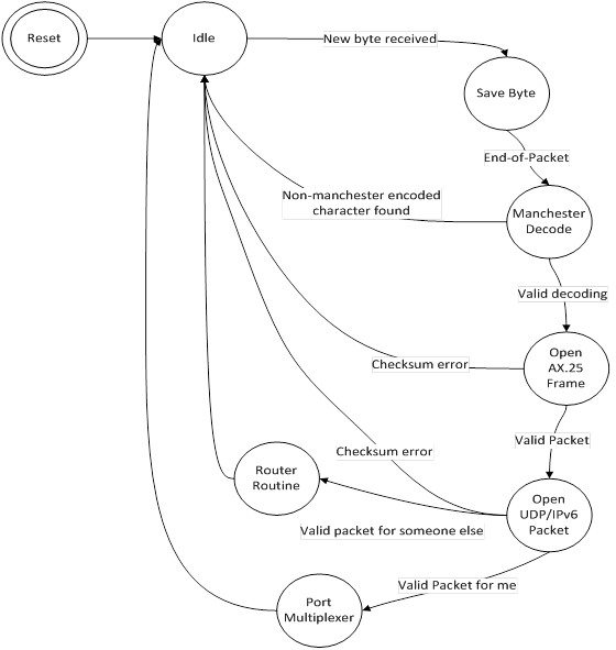
Figure 24 Radiotftp_process Receive FSM diagram
|
|
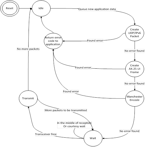
Figure 25 Radiotftp_process send FSM diagram
|
#include <stdio.h> #include <avr/io.h> #include <avr/iom128rfa1.h> #include <avr/interrupt.h> #include <util/delay.h>
#include "contiki.h" #include "contiki-conf.h" #include "contiki-net.h" #include "contiki-lib.h" #include "dev/rs232.h" #include "radiotftp.h"
PROCESS(measurement_process, "Measurement Process"); AUTOSTART_PROCESSES(&measurement_process, &radiotftp_process);
PROCESS_THREAD(measurement_process, ev, data) { static uint32_t counter=0; static uint16_t numBytes=0; static uint64_t fibo[3] = {0, 1, 1}; static struct etimer measurement_timer; static uint8_t fake_measurement_string[450]; PROCESS_BEGIN();
etimer_set(&measurement_timer, CLOCK_SECOND*2); while(1) { PROCESS_WAIT_EVENT(); counter++; fibo[2]=fibo[1]+fibo[0]; numBytes=sprintf(fake_measurement_string, "Some Data: fibonacci(%d)=", counter); numBytes+=sprintf(fake_measurement_string+numBytes, "%u [Alp Sayin, KTH Royal Institute of Technology]\n", fibo[0]); printf("%s", fake_measurement_string); fibo[0]=fibo[1]; fibo[1]=fibo[2]; radiotftp_setNumBytesToSend(numBytes); process_post_synch( &radiotftp_process, PROCESS_EVENT_COM, (void*)fake_measurement_string); etimer_set(&measurement_timer, CLOCK_SECOND*10); } PROCESS_END(); }
|
Figure 26 Sample Contiki Process computing Fibonacci Series
|
#include <stdio.h> #include <stdlib.h> #include <string.h> #include <unistd.h> #include <net/if.h> #include <linux/if_tun.h> #include <sys/types.h> #include <sys/socket.h> #include <sys/ioctl.h> #include <sys/stat.h> #include <fcntl.h> #include <arpa/inet.h> #include <sys/select.h> #include <sys/time.h> #include <errno.h> #include <stdarg.h>
#include "tun_alloc.h"
int tun_alloc(char* dev, int flags) { struct ifreq ifr; int fd, err; char* clonedev = "/dev/net/tun"; if((fd = open(clonedev, O_RDWR)) < 0) { return fd; } memset(&ifr, 0, sizeof(ifr));
ifr.ifr_flags = flags; //IF_TUN or IFF_TAP, plus maybe IFF_NO_PI if(*dev) { strncpy(ifr.ifr_name, dev, IFNAMSIZ); } if((err = ioctl(fd, TUNSETIFF, (void*) &ifr)) < 0) { close(fd); return err; } strcpy(dev, ifr.ifr_name); return fd; } |
Figure 27 Code segment from tun_alloc.c, demonstrating the opening procedure of a Tun device
|
//TUNTAP DEVICE if (FD_ISSET(tun_fd, &rfds)) { nread = read(tun_fd, read_buffer, sizeof(read_buffer)); if (nread < 0) { perror("Reading from if interface"); close(tun_fd); exit(EXIT_FAILURE); } printf("Read %d bytes from device %s\n", nread, tun_name); printAsciiHex(read_buffer, nread); /* * ping modifier for 10.0.0.4 * simply swaps the last bytes of the ping packet's source and destination ips * and writes it back by setting the ICMP type 0 */ #if 1 for (i = 0; i < MODIFY_LIST_LENGTH; i++) { if (!memcmp(read_buffer + 16, modify[i], 4)) //ip match { if (read_buffer[9] == 1 && read_buffer[1] == 0) { if (read_buffer[20] == 8 && read_buffer[21] == 0) { read_buffer[nread] = read_buffer[15]; read_buffer[12] = 10; //src read_buffer[13] = 0; //src read_buffer[14] = 1; //src read_buffer[15] = 2; //src read_buffer[16] = 10; //dst read_buffer[17] = 0; //dst read_buffer[18] = 1; //dst read_buffer[19] = 1; //dst // read_buffer[20] = 0; write(tun_fd, read_buffer, nread); } } } } #endif |
Figure 28 Ping responder code segment from tunclient.c
|
int telemetry_postpoll(struct aprxpolls *app) { #if 0 if (telemetry_time <= now.tv_sec) { telemetry_time += telemetry_interval; if (telemetry_time <= now.tv_sec) telemetry_time = now.tv_sec + telemetry_interval; telemetry_datatx(); }
if (telemetry_labeltime <= now.tv_sec) { telemetry_labeltime += telemetry_labelinterval; if (telemetry_labeltime <= now.tv_sec) telemetry_labeltime = now.tv_sec + 120; telemetry_labeltx(); } #endif return 0; } |
Figure 29 A simple fix to disable automated telemetry messages of aprx (function extracted from telemetry.c).
|
k=0 analog_value=16 digital_value=1 while : telemetrit label SA0BXI SA0BXI-13 ANVAL NA NA NA NA DIG > /tmp/wxbeacon.txt sleep 61 telemetrit coef SA0BXI SA0BXI-13 0 1 0 > /tmp/wxbeacon.txt sleep 61 do for((i=0; i<4; i++)) do telemetrit data SA0BXI SA0BXI-13 $k $analog_value 0 0 0 0 $digital_value > /tmp/wxbeacon.txt sleep 61 done done |
Figure 30 A simple shell script to automate the transmission of data as APRS telemetry
|
$time [helloWorld->] |
Program Start |
|
$time [TX->enabled] |
TX enabled/RX disabled |
|
$time [RX->enabled] |
RX enabled/TX disabled |
|
$time [wrq_request->$file] |
Received wrq request for $file |
|
$time [connectionclose->$cause] |
Connection closed due to $cause |
|
$time [connection_cancel->$cause] |
Connection canceled due to $cause |
|
$time [put->$file] |
Sent wrq request for $file |
|
$time [exit->] |
Program exit |
|
$time [RETRANSMIT->$type] |
Retransmitting $type of packet |
Table 4 Sample Log Format
|
1341681601.774328 [put->text2k.txt] 1341681601.874703 [TX->enabled] 1341681602.318331 [RX->enabled] 1341681602.759087 [TX->enabled] 1341681603.761352 [RX->enabled] 1341681604.787046 [RETRANSMIT->data] 1341681604.887233 [TX->enabled] 1341681605.881348 [RX->enabled] 1341681606.915194 [RETRANSMIT->data] 1341681607.015385 [TX->enabled] 1341681608.013341 [RX->enabled] 1341681609.043301 [RETRANSMIT->data] 1341681609.143489 [TX->enabled] 1341681610.137347 [RX->enabled] 1341681613.171422 [RETRANSMIT->data] 1341681613.271607 [TX->enabled] 1341681614.274311 [RX->enabled] 1341681616.299526 [RETRANSMIT->data] 1341681616.399711 [TX->enabled] 1341681617.395334 [RX->enabled] 1341681620.427672 [RETRANSMIT->data] 1341681620.527878 [TX->enabled] 1341681621.517350 [RX->enabled] 1341681623.555803 [RETRANSMIT->data] 1341681623.656008 [TX->enabled] 1341681624.627345 [RX->enabled] 1341681625.685871 [RETRANSMIT->data] 1341681625.786058 [TX->enabled] 1341681626.776325 [RX->enabled] 1341681629.813999 [RETRANSMIT->data] 1341681629.914199 [TX->enabled] 1341681630.910356 [RX->enabled] 1341681632.945202 [exit->] |
Table 5 Sample event log extract
|
Data |
Value |
Unit |
|
Transfer Time |
2.4141 |
seconds |
|
Bitrate |
52.6076 |
Bytes/second |
|
Latency |
0.019 |
Seconds/byte |
|
Ideal number of transmissions |
2 |
Packets |
|
Number of transmissions |
2 |
Packets |
|
Number of receptions |
2 |
Packets |
|
Number of retransmissions |
0 |
Packets |
|
Tx Enabled Time |
1.2999 |
Seconds |
|
Rx Enabled Time |
1.1141 |
Seconds |
|
Error Rate |
0 |
Percent |
|
Success Rate |
0 |
Percent |
|
Energy Consumption |
0.6212 |
Joules |
|
Number of Samples |
5 |
Transfers |
|
Number of Disconnects |
0 |
Transfers |
Table 6 Results of transfer experiments with 127 bytes in location 0.
|
Data |
Value |
Unit |
|
Transfer Time |
2.4172 |
seconds |
|
Bitrate |
52.5401 |
Bytes/second |
|
Latency |
0.019 |
Seconds/bit |
|
Ideal number of transmissions |
2 |
Packets |
|
Number of transmissions |
2 |
Packets |
|
Number of receptions |
2 |
Packets |
|
Number of retransmissions |
0 |
Packets |
|
Tx Enabled Time |
1.2896 |
Seconds |
|
Rx Enabled Time |
1.1276 |
Seconds |
|
Error Rate |
0 |
Percent |
|
Success Rate |
0 |
Percent |
|
Energy Consumption |
0.6189 |
Joules |
|
Number of Transfers |
6 |
Transfers |
|
Number of Disconnects |
0 |
Transfers |
Table 7 Results of transfer experiments with 127 bytes from location 1.
|
Data |
Value |
Unit |
|
Transfer Time |
5.8604 |
seconds |
|
Bitrate |
21.6709 |
Bytes/second |
|
Latency |
0.0461 |
Seconds/bit |
|
Ideal number of transmissions |
2 |
Packets |
|
Number of transmissions |
2.8889 |
Packets |
|
Number of receptions |
2.8889 |
Packets |
|
Number of retransmissions |
0.8889 |
Packets |
|
Tx Enabled Time |
1.8603 |
Seconds |
|
Rx Enabled Time |
4.0001 |
Seconds |
|
Error Rate |
0.2037 |
Percent |
|
Success Rate |
0.7963 |
percent |
|
Energy Consumption |
1.1776 |
Joules |
|
Number of Transfers |
11 |
Transfers |
|
Number of Disconnects |
2 |
Transfers |
Table 8 Results of transfer experiments with 127 bytes from location 2.
|
Data |
Value |
Unit |
|
Transfer Time |
6.6321 |
seconds |
|
Bitrate |
19.1493 |
Bytes/second |
|
Latency |
0.0522 |
Seconds/bit |
|
Ideal number of transmissions |
2 |
Packets |
|
Number of transmissions |
3.1429 |
Packets |
|
Number of receptions |
3.1429 |
Packets |
|
Number of retransmissions |
1.1429 |
Packets |
|
Tx Enabled Time |
2.0248 |
Seconds |
|
Rx Enabled Time |
4.6073 |
Seconds |
|
Error Rate |
0.1557 |
Percent |
|
Success Rate |
0.8443 |
percent |
|
Energy Consumption |
1.3122 |
Joules |
|
Number of Transfers |
18 |
Transfers |
|
Number of Disconnects |
4 |
Transfers |
Table 9 Results of transfer experiments with 127 bytes from location 3.
|
Data |
Value |
Unit |
|
Transfer Time |
3.6759 |
seconds |
|
Bitrate |
34.5494 |
Bytes/second |
|
Latency |
0.0289 |
Seconds/bit |
|
Ideal number of transmissions |
2 |
Packets |
|
Number of transmissions |
2.3333 |
Packets |
|
Number of receptions |
2.3333 |
Packets |
|
Number of retransmissions |
0.3333 |
Packets |
|
Tx Enabled Time |
1.5393 |
Seconds |
|
Rx Enabled Time |
2.1365 |
Seconds |
|
Error Rate |
0.1111 |
Percent |
|
Success Rate |
0.8889 |
percent |
|
Energy Consumption |
0.8336 |
Joules |
|
Number of Transfers |
14 |
Transfers |
|
Number of Disconnects |
2 |
Transfers |
Table 10 Results of transfer experiments with 127 bytes from location 4.
|
Data |
Value |
Unit |
|
Transfer Time |
N/A |
seconds |
|
Bitrate |
N/A |
Bytes/second |
|
Latency |
N/A |
Seconds/bit |
|
Ideal number of transmissions |
2 |
Packets |
|
Number of transmissions |
N/A |
Packets |
|
Number of receptions |
N/A |
Packets |
|
Number of retransmissions |
N/A |
Packets |
|
Tx Enabled Time |
N/A |
Seconds |
|
Rx Enabled Time |
N/A |
Seconds |
|
Error Rate |
N/A |
Percent |
|
Success Rate |
N/A |
percent |
|
Energy Consumption |
N/A |
Joules |
|
Number of Transfers |
4 |
Transfers |
|
Number of Disconnects |
4 |
Transfers |
Table 11 Results of transfer experiments with 127 bytes from location 5.
|
Data |
Value |
Unit |
|
Transfer Time |
3.1727 |
seconds |
|
Bitrate |
40.0290 |
Bytes/second |
|
Latency |
0.0250 |
Seconds/bit |
|
Ideal number of transmissions |
2 |
Packets |
|
Number of transmissions |
2.2000 |
Packets |
|
Number of receptions |
2.2000 |
Packets |
|
Number of retransmissions |
0.2000 |
Packets |
|
Tx Enabled Time |
1.4162 |
Seconds |
|
Rx Enabled Time |
1.7565 |
Seconds |
|
Error Rate |
0.0667 |
Percent |
|
Success Rate |
0.9333 |
percent |
|
Energy Consumption |
0.7419 |
Joules |
|
Number of Transfers |
17 |
Transfers |
|
Number of Disconnected |
2 |
Transfers |
Table 12 Results of transfer experiments with 127 bytes from location 6.
|
Data |
Value |
Unit |
|
Transfer Time |
4.1403 |
seconds |
|
Bitrate |
30.6741 |
Bytes/second |
|
Latency |
0.0326 |
Seconds/bit |
|
Ideal number of transmissions |
2 |
Packets |
|
Number of transmissions |
2.4667 |
Packets |
|
Number of receptions |
2.4667 |
Packets |
|
Number of retransmissions |
0.4667 |
Packets |
|
Tx Enabled Time |
1.6138 |
Seconds |
|
Rx Enabled Time |
2.5266 |
Seconds |
|
Error Rate |
14.44 |
Percent |
|
Success Rate |
85.56 |
percent |
|
Energy Consumption |
0.9083 |
Joules |
|
Number of Transfers |
15 |
Transfers |
|
Number of Disconnects |
0 |
Transfers |
Table 13 Results of transfer experiments with 127 bytes from location 7.
|
Data |
Value |
Unit |
|
Transfer Time |
21.7267 |
seconds |
|
Bitrate |
94.2619 |
Bytes/second |
|
Latency |
0.0106 |
Seconds/bit |
|
Ideal number of transmissions |
16 |
Packets |
|
Number of transmissions |
16 |
Packets |
|
Number of receptions |
16 |
Packets |
|
Number of retransmissions |
0 |
Packets |
|
Tx Enabled Time |
14.7241 |
Seconds |
|
Rx Enabled Time |
7.0026 |
Seconds |
|
Error Rate |
0 |
Percent |
|
Success Rate |
1 |
percent |
|
Energy Consumption |
6.3618 |
Joules |
|
Number of Transfers |
6 |
Transfers |
|
Number of Disconnects |
1 |
Transfers |
Table 14 Results of transfer experiments with 2 kbytes in location 0.
|
Data |
Value |
Unit |
|
Transfer Time |
21.7249 |
seconds |
|
Bitrate |
94.2697 |
Bytes/second |
|
Latency |
0.0106 |
Seconds/bit |
|
Ideal number of transmissions |
16 |
Packets |
|
Number of transmissions |
16 |
Packets |
|
Number of receptions |
16 |
Packets |
|
Number of retransmissions |
0 |
Packets |
|
Tx Enabled Time |
14.5769 |
Seconds |
|
Rx Enabled Time |
7.1480 |
Seconds |
|
Error Rate |
0 |
Percent |
|
Success Rate |
1 |
percent |
|
Energy Consumption |
6.3241 |
Joules |
|
Number of Transfers |
7 |
Transfers |
|
Number of Disconnects |
1 |
Transfers |
Table 15 Results of transfer experiments with 2 kbytes from location 1.
|
Data |
Value |
Unit |
|
Transfer Time |
22.6350 |
seconds |
|
Bitrate |
90.4793 |
Bytes/second |
|
Latency |
0.0111 |
Seconds/bit |
|
Ideal number of transmissions |
16 |
Packets |
|
Number of transmissions |
16.3333 |
Packets |
|
Number of receptions |
16.3333 |
Packets |
|
Number of retransmissions |
0.3333 |
Packets |
|
Tx Enabled Time |
14.8774 |
Seconds |
|
Rx Enabled Time |
7.7576 |
Seconds |
|
Error Rate |
0.0196 |
Percent |
|
Success Rate |
0.9804 |
percent |
|
Energy Consumption |
6.5099 |
Joules |
|
Number of Transfers |
7 |
Transfers |
|
Number of Disconnects |
1 |
Transfers |
Table 16 Results of transfer experiments with 2 kbytes from location 2.
|
Data |
Value |
Unit |
|
Transfer Time |
22.7599 |
seconds |
|
Bitrate |
89.9828 |
Bytes/second |
|
Latency |
0.0111 |
Seconds/bit |
|
Ideal number of transmissions |
16 |
Packets |
|
Number of transmissions |
16.2857 |
Packets |
|
Number of receptions |
16.2857 |
Packets |
|
Number of retransmissions |
0.2857 |
Packets |
|
Tx Enabled Time |
14.7559 |
Seconds |
|
Rx Enabled Time |
8.0039 |
Seconds |
|
Error Rate |
0.0168 |
Percent |
|
Success Rate |
0.9832 |
percent |
|
Energy Consumption |
6.4940 |
Joules |
|
Number of Transfers |
7 |
Transfers |
|
Number of Disconnects |
0 |
Transfers |
Table 17 Results of transfer experiments with 2 kbytes from location 3.
|
Data |
Value |
Unit |
|
Transfer Time |
23.1693 |
seconds |
|
Bitrate |
88.3928 |
Bytes/second |
|
Latency |
0.0113 |
Seconds/bit |
|
Ideal number of transmissions |
16 |
Packets |
|
Number of transmissions |
16.5 |
Packets |
|
Number of receptions |
16.5 |
Packets |
|
Number of retransmissions |
0.6250 |
Packets |
|
Tx Enabled Time |
14.8603 |
Seconds |
|
Rx Enabled Time |
8.3090 |
Seconds |
|
Error Rate |
0.0359 |
Percent |
|
Success Rate |
0.9714 |
percent |
|
Energy Consumption |
6.5697 |
Joules |
|
Number of Transfers |
8 |
Transfers |
|
Number of Disconnects |
0 |
Transfers |
Table 18 Results of transfer experiments with 2 kbytes from location 4.
|
Data |
Value |
Unit |
|
Transfer Time |
N/A |
seconds |
|
Bitrate |
N/A |
Bytes/second |
|
Latency |
N/A |
Seconds/bit |
|
Ideal number of transmissions |
16 |
Packets |
|
Number of transmissions |
N/A |
Packets |
|
Number of receptions |
N/A |
Packets |
|
Number of retransmissions |
N/A |
Packets |
|
Tx Enabled Time |
N/A |
Seconds |
|
Rx Enabled Time |
N/A |
Seconds |
|
Error Rate |
N/A |
Percent |
|
Success Rate |
N/A |
percent |
|
Energy Consumption |
N/A |
Joules |
|
Number of Transfers |
3 |
Transfers |
|
Number of Disconnects |
3 |
Transfers |
Table 19 Results of transfer experiments with 2 kbytes from location 5.
|
Data |
Value |
Unit |
|
Transfer Time |
22.1851 |
seconds |
|
Bitrate |
92.3142 |
Bytes/second |
|
Latency |
0.0108 |
Seconds/bit |
|
Ideal number of transmissions |
16 |
Packets |
|
Number of transmissions |
16.1111 |
Packets |
|
Number of receptions |
16.1111 |
Packets |
|
Number of retransmissions |
0.1111 |
Packets |
|
Tx Enabled Time |
14.6391 |
Seconds |
|
Rx Enabled Time |
7.5460 |
Seconds |
|
Error Rate |
0.0065 |
Percent |
|
Success Rate |
0.9935 |
percent |
|
Energy Consumption |
6.3952 |
Joules |
|
Number of Transfers |
9 |
Transfers |
|
Number of Disconnects |
0 |
Transfers |
Table 20 Results of transfer experiments with 2 kbytes from location 6.
|
Data |
Value |
Unit |
|
Transfer Time |
23.5792 |
seconds |
|
Bitrate |
86.8562 |
Bytes/second |
|
Latency |
0.0115 |
Seconds/bit |
|
Ideal number of transmissions |
16 |
Packets |
|
Number of transmissions |
16.6250 |
Packets |
|
Number of receptions |
16.6250 |
Packets |
|
Number of retransmissions |
0.6250 |
Packets |
|
Tx Enabled Time |
14.9375 |
Seconds |
|
Rx Enabled Time |
8.6418 |
Seconds |
|
Error Rate |
0.0344 |
Percent |
|
Success Rate |
0.9656 |
percent |
|
Energy Consumption |
6.6386 |
Joules |
|
Number of Transfers |
8 |
Transfers |
|
Number of Disconnects |
0 |
Transfers |
Table 21 Results of transfer experiments with 2 kbytes from location 7.
|
Data |
Value |
Unit |
|
Transfer Time |
0.8727 |
seconds |
|
Bitrate |
145.5254 |
Bytes/second |
|
Latency |
0.0069 |
Seconds/bit |
|
Ideal number of transmissions |
2 |
Packets |
|
Number of transmissions |
2 |
Packets |
|
Number of receptions |
2 |
Packets |
|
Number of retransmissions |
0 |
Packets |
|
Tx Enabled Time |
0.3297 |
Seconds |
|
Rx Enabled Time |
0.5430 |
Seconds |
|
Error Rate |
0 |
Percent |
|
Success Rate |
1 |
percent |
|
Energy Consumption |
0.0584 |
Joules |
|
Number of Transfers |
10 |
Transfers |
|
Number of Disconnects |
2 |
Transfers |
Table 22 Results of transfer experiments with 127 bytes in location 0.
|
Data |
Value |
Unit |
|
Transfer Time |
6.6522 |
seconds |
|
Bitrate |
19.0914 |
Bytes/second |
|
Latency |
0.0524 |
Seconds/bit |
|
Ideal number of transmissions |
2 |
Packets |
|
Number of transmissions |
4.1875 |
Packets |
|
Number of receptions |
4.1875 |
Packets |
|
Number of retransmissions |
2.1875 |
Packets |
|
Tx Enabled Time |
0.6610 |
Seconds |
|
Rx Enabled Time |
5.9912 |
Seconds |
|
Error Rate |
0.3346 |
Percent |
|
Success Rate |
0.6654 |
percent |
|
Energy Consumption |
0.3670 |
Joules |
|
Number of Transfers |
21 |
Transfers |
|
Number of Disconnects |
5 |
Transfers |
Table 23 Results of transfer experiments with 127 bytes from location 1.
|
Data |
Value |
Unit |
|
Transfer Time |
N/A |
seconds |
|
Bitrate |
N/A |
Bytes/second |
|
Latency |
N/A |
Seconds/bit |
|
Ideal number of transmissions |
2 |
Packets |
|
Number of transmissions |
N/A |
Packets |
|
Number of receptions |
N/A |
Packets |
|
Number of retransmissions |
N/A |
Packets |
|
Tx Enabled Time |
N/A |
Seconds |
|
Rx Enabled Time |
N/A |
Seconds |
|
Error Rate |
N/A |
Percent |
|
Success Rate |
N/A |
percent |
|
Energy Consumption |
N/A |
Joules |
|
Number of Transfers |
10 |
Transfers |
|
Number of Disconnects |
10 |
Transfers |
Table 24 Results of transfer experiments with 127 bytes from location 2.
|
Data |
Value |
Unit |
|
Transfer Time |
11.5138 |
seconds |
|
Bitrate |
11.0302 |
Bytes/second |
|
Latency |
0.0907 |
Seconds/bit |
|
Ideal number of transmissions |
2 |
Packets |
|
Number of transmissions |
7 |
Packets |
|
Number of receptions |
7 |
Packets |
|
Number of retransmissions |
5 |
Packets |
|
Tx Enabled Time |
1.0969 |
Seconds |
|
Rx Enabled Time |
10.4168 |
Seconds |
|
Error Rate |
0.7143 |
Percent |
|
Success Rate |
0.2857 |
percent |
|
Energy Consumption |
0.6333 |
Joules |
|
Number of Transfers |
7 |
Transfers |
|
Number of Disconnects |
6 |
Transfers |
Table 25 Results of transfer experiments with 127 bytes from location 4.
|
Data |
Value |
Unit |
|
Transfer Time |
8.9151 |
seconds |
|
Bitrate |
229.7226 |
Bytes/second |
|
Latency |
0.0044 |
Seconds/bit |
|
Ideal number of transmissions |
16 |
Packets |
|
Number of transmissions |
16.6667 |
Packets |
|
Number of receptions |
16.6667 |
Packets |
|
Number of retransmissions |
0.6667 |
Packets |
|
Tx Enabled Time |
3.8002 |
Seconds |
|
Rx Enabled Time |
5.1149 |
Seconds |
|
Error Rate |
0.0326 |
Percent |
|
Success Rate |
0.9674 |
percent |
|
Energy Consumption |
0.6143 |
Joules |
|
Number of Transfers |
16 |
Transfers |
|
Number of Disconnects |
1 |
Transfers |
Table 26 Results of transfer experiments with 2 kbytes in location 0.
|
Data |
Value |
Unit |
|
Transfer Time |
N/A |
seconds |
|
Bitrate |
N/A |
Bytes/second |
|
Latency |
N/A |
Seconds/bit |
|
Ideal number of transmissions |
16 |
Packets |
|
Number of transmissions |
N/A |
Packets |
|
Number of receptions |
N/A |
Packets |
|
Number of retransmissions |
N/A |
Packets |
|
Tx Enabled Time |
N/A |
Seconds |
|
Rx Enabled Time |
N/A |
Seconds |
|
Error Rate |
N/A |
Percent |
|
Success Rate |
N/A |
percent |
|
Energy Consumption |
N/A |
Joules |
|
Number of Transfers |
5 |
Transfers |
|
Number of Disconnects |
5 |
Transfers |
Table 27 Results of transfer experiments with 2 kbytes from location 1.
|
Data |
Value |
Unit |
|
Transfer Time |
N/A |
seconds |
|
Bitrate |
N/A |
Bytes/second |
|
Latency |
N/A |
Seconds/bit |
|
Ideal number of transmissions |
16 |
Packets |
|
Number of transmissions |
N/A |
Packets |
|
Number of receptions |
N/A |
Packets |
|
Number of retransmissions |
N/A |
Packets |
|
Tx Enabled Time |
N/A |
Seconds |
|
Rx Enabled Time |
N/A |
Seconds |
|
Error Rate |
N/A |
Percent |
|
Success Rate |
N/A |
percent |
|
Energy Consumption |
N/A |
Joules |
|
Number of Transfers |
4 |
Transfers |
|
Number of Disconnects |
4 |
Transfers |
Table 28 Results of transfer experiments with 2 kbytes from location 2.
|
Data |
Value |
Unit |
|
Transfer Time |
N/A |
seconds |
|
Bitrate |
N/A |
Bytes/second |
|
Latency |
N/A |
Seconds/bit |
|
Ideal number of transmissions |
16 |
Packets |
|
Number of transmissions |
N/A |
Packets |
|
Number of receptions |
N/A |
Packets |
|
Number of retransmissions |
N/A |
Packets |
|
Tx Enabled Time |
N/A |
Seconds |
|
Rx Enabled Time |
N/A |
Seconds |
|
Error Rate |
N/A |
Percent |
|
Success Rate |
N/A |
percent |
|
Energy Consumption |
N/A |
Joules |
|
Number of Transfers |
4 |
Transfers |
|
Number of Disconnects |
4 |
Transfers |
Table 29 Results of transfer experiments with 2 kbytes from location 4.